Spatio-temporal segregation of brain
circuitries activated during movie
viewing
Low Temperature Laboratory, Brain Research Unit
Department of Biomedical Engineering and Computational Science
Thesis submitted for examination for the degree of Master of Science in Technology.
Espoo March 11th, 2011
Thesis supervisor:
Prof. Mikko Sams
Thesis instructors:
D.Sc. (Tech.) Sanna Malinen Academy Professor Riitta Hari
A
?
Aalto UniversityAuthor: Siina Pamilo
Title: Spatio-temporal segregation of brain circuitries activated during movie viewing
Date: March 11th, 2011 Language: English Number of pages:9+50 Low Temperature Laboratory, Brain Research Unit
Department of Biomedical Engineering and Computational Science
Professorship: Cognitive technology Code: S-114
Supervisor: Prof. Mikko Sams
Instructors: D.Sc. (Tech.) Sanna Malinen, Academy Professor Riitta Hari
So called resting state networks (RSNs), i.e. functionally connected brain areas that are active both during rest and task conditions, are receiving growing atten-tion in modern brain research. The first observed RSN was the motor network. Since then, several different cortical networks have been identified. In this thesis the focus was on the sensorimotor, dorsal attention and default-mode networks.
Independent component analysis (ICA) was used to segregate the three cor-tical networks from fMRI data collected from 15 subjects who were watching a 15 minutes long film (”At land” by Maya Deren). ICA was performed at three different dimensionalities and the effect of increasing the number of component estimates was examined. The functional connectivity between brain areas occu-pied by the three networks was examined also with seed-based correlation. The stimulus-related brain areas were indentified with intersubject correlation (ISC) analysis and the ICs were sorted according to the spatial overlap with the ISC map. The time courses of the most stimulus related ICs were compared with events in the movie.
At a low dimensionality of ICA (25), the ICs representing the sensorimotor and dorsal attention networks included brain areas that do not belong to the networks. With an intermediate number of components (40) the additional areas were sepa-rated from the networks. This dimensionality was apparently closest to the correct one. When the dimensionality was further increased (70), the networks split into subcomponents. Although the spatial splitting was physiologically sensible, the time courses of the ICs got distorted at a too high dimensionality. The results of this work contribute to understanding how the number of components affects the group-ICA results and how the correct number of ICs could be empirically controlled in group-fMRI data.
Keywords: fMRI, ICA, seed-based correlation, ISC, RSN, naturalistic stimula-tion, human brain, movie
Tekij¨a: Siina Pamilo
Ty¨on nimi: Elokuvan katselun aktivoimien aivoverkostojen ajallispaikallinen erottelu
P¨aiv¨am¨a¨ar¨a: 11.3.2011 Kieli: Englanti Sivum¨a¨ar¨a:9+50 Kylm¨alaboratorio, Aivotutkimusyksikk¨o
L¨a¨aketieteellisen tekniikan ja laskennallisen tieteen laitos
Professuuri: Kognitiivinen teknologia Koodi: S-114 Valvoja: Prof. Mikko Sams
Ohjaajat: TkT Sanna Malinen, Akatemiaprofessori Riitta Hari
Niin levon kuin teht¨av¨an suorituksen aikana aktiiviset, toisiinsa toiminnallises-ti kytkeytyneet aivoalueet, eli nk. lepoverkostot, ovat yksi nykyaikaisen aivo-tutkimuksen erityisist¨a mielenkiinnon kohteista. Ensimm¨aiseksi havaittiin mo-torinen verkosto, mink¨a j¨alkeen on l¨oydetty monia muita aivoverkostoja. T¨ass¨a diplomity¨oss¨a tutkittiin sensorimotorista ja dorsaalista tarkkaavaisuus verkostoa sek¨a nk. default mode -verkostoa.
N¨am¨a kolme aivoverkostoa erotettiin 15 minuutin pituisen elokuvan (”At Land”, Maya Deren) katselun aikana 15 koehenkil¨olt¨a ker¨atyst¨a fMRI-datasta riippumattomien komponenttien analyysill¨a (ICA). Estimoitujen riippumattomien komponenttien (IC) lukum¨a¨ar¨an vaikutusta ryhm¨a-ICAn tuloksiin tarkasteltiin kolmella eri komponenttim¨a¨ar¨all¨a. ICAlla l¨oydettyjen aivoverkostojen toiminnalli-nen yhteys todettiin my¨os l¨ahdekorrelaatiomenetelm¨all¨a. Korrelaatioanalyysin (ISC) avulla paikannettiin ¨arsykkeeseen liittyv¨at aivoalueet ja ICt j¨arjestettiin ISC-kartan avulla. N¨ain pystyttiin tunnistamaan ¨arsykkeeseen reagoivat kompo-nentit, joiden aikasarjoja verrattiin elokuvan tapahtumiin.
Pienell¨a komponenttim¨a¨ar¨all¨a (25) sensorimotorista ja tarkkaavaisuusverkos-toa vastaavat komponentit sis¨alsiv¨at my¨os n¨aihin verkostoihin kuulumattomia aivoalueita. Kun komponenttim¨a¨ar¨a¨a kasvatettiin (40), ylim¨a¨ar¨aiset alueet erot-tuivat omiksi verkostoikseen, josta voitiin olettaa, ett¨a t¨am¨a komponenttim¨a¨ar¨a oli l¨ahell¨a oikeaa. Suurella komponenttim¨a¨ar¨all¨a (70) aivoverkostot jakaantuivat pienempiin osiin. Vaikka spatiaalinen jakaantuminen oli fysiologisesti mielek¨ast¨a, komponenttien aikasarjat v¨a¨aristyiv¨at liian suurella komponenttim¨a¨ar¨all¨a. T¨am¨an ty¨on tulokset auttavat ymm¨art¨am¨a¨an, miten riippumattomien komponenttien lukum¨a¨ar¨a vaikuttaa ryhm¨a-ICAn tuloksiin. Tuloksia voidaan soveltaa oikean komponenttim¨a¨ar¨an kokeellisessa etsimisess¨a ryhm¨a-fMRI datasta.
Avainsanat: fMRI, ICA, l¨ahdekorrelaatio, korrelaatioanalyysi, lepoverkosto, luonnonmukainen ¨arsyke, aivot, elokuva
Preface
This work was done in collaboration with the aivoAALTO project at the Brain Research Unit of the Low Temperature Laboratory (LTL) and at the Advanced Magnetic Imaging Centre (AMI) of the Aalto University School of Science. I would like to thank my instructors Sanna Malinen and Riitta Hari for their patient guid-ance and expert advice. I am also grateful to my supervisor Mikko Sams for allowing me to choose this interesting topic for my thesis. My sincere thanks goes to Yevhen Hlushchuk, Pia Tikka and Marita Kattelus for fMRI data collection. Special thanks goes to Yevhen for his help in pre-processing of the data and to Ville Renvall for his constructive comments related to MRI physics. Finally, I owe my deepest gratitude to my family and friends for support and encouragement.
Otaniemi, March 11th, 2011
Contents
Abstract ii
Abstract (in Finnish) iii
Preface iv
Contents v
Symbols and abbreviations vii
1 Introduction 1
2 Spontaneous BOLD fluctuations in the human brain 2
3 Naturalistic stimulation in fMRI 5
4 Number of independent sources in fMRI data 6
5 Magnetic resonance imaging 7
5.1 A short history of MRI . . . 7
5.2 Nuclear spins . . . 8
5.3 Net magnetization . . . 9
5.4 Radio-frequency excitation . . . 9
5.5 Gradient fields. . . 10
5.6 Pulse sequences and image contrast . . . 11
5.7 Functional magnetic resonance imaging . . . 14
5.7.1 The BOLD effect . . . 14
5.7.2 Echo planar imaging . . . 14
5.7.3 The haemodynamic response. . . 15
6 Analysis of fMRI data 16 6.1 Pre-processing of images . . . 16 6.1.1 Slice-timing correction . . . 16 6.1.2 Realignment . . . 16 6.1.3 Coregistration . . . 16 6.1.4 Spatial normalization . . . 17 6.1.5 Spatial smoothing. . . 17
6.2 The general linear model . . . 17
6.3 Inter-subject correlation . . . 18
6.4 Seed-based correlation . . . 18
6.5 Independent component analysis. . . 18
6.5.1 Motivation. . . 18
6.5.2 Definition of ICA . . . 19
6.5.3 Measures of non-gaussianity . . . 20
6.5.5 Ambiguities of ICA . . . 22
6.5.6 ICASSO . . . 22
6.5.7 Application of ICA to fMRI data . . . 22
6.5.8 Group ICA . . . 22
7 Materials and methods 24 7.1 Subjects . . . 24
7.2 Stimuli . . . 24
7.3 Data acquisition. . . 24
7.4 Pre-processing . . . 25
7.5 ICA . . . 25
7.6 Sorting of components using inter-subject correlation . . . 25
7.7 Seed-based correlation . . . 26
8 Results 27 8.1 Brain areas comprising the sensorimotor network . . . 27
8.2 Brain areas comprising the attention network . . . 27
8.3 Brain areas comprising the default-mode network . . . 31
8.4 ICASSO results . . . 31
8.5 IC time courses . . . 32
8.5.1 Correlations between the IC time courses . . . 32
8.5.2 IC time courses and the extracted fMRI signal . . . 34
8.6 Single-subject ICA . . . 35
8.7 ICASSO analysis with subjects in different concatenation order . . . 35
8.8 IC ordering using the ISC map . . . 35
8.9 Relation to events in the movie . . . 36
8.10 Seed-based correlation . . . 38
9 Discussion and conclusions 40 9.1 Effect of the number of ICs on group ICA results . . . 40
9.2 Temporal activation patterns of the ICs. . . 42
Symbols and abbreviations
Symbols
~B0 Magnetic field strength ~
J Angular momentum ~
M Magnetization ~
µ Dipole magnetic moment γ Gyromagnetic ratio
~ Reduced Planck’s constant
ω0 Larmor frequency
ωRF Angular frequency of radio-frequency radiation
s Spin quantum number ms Magnetic quantum number
E↑ Energy of spins aligned with the external magnetic field
E↓ Energy of spins aligned anti-parallel to the external magnetic field
ERF Energy of the radio-frequency radiation
T1 Time constant for longitudial relaxation T2 Time constant for transversal relaxation
T2∗ Time constant for enhanced transversal relaxation
T2′ Time constant for transversal relaxation caused by field inhomogeneities βi ith parameter weight
gi ith covariate ǫ Error term X Measured data e X Whitened data A Mixing matrix e
A Whitened mixing matrix W Inverse of the mixing matrix S Independent components
E Orthogonal matrix of eigenvectors D Diagonal matrix of eigenvalues Θk Model parameter ofkth order
λi ith eigenvalue
Fi Reducing matrix for subject i
G Reducing matrix for the concatenated data set ˆ
A Mixing matrix for group data ˆ
Operators
E{·} Expectation F {·} Fourier transform H(·) Entropy I(·) Mutual information L(·) Maximum log-likelihoodG(·) Penalty term for model complexity
P
i Sum over index i
Q
Abbreviations
BOLD Blood oxygen level dependent (signal) CBF Cerebral blood flow
CMRO2 Cerebral metabolic rate of oxygen consumption DAQ Data aquisition
DMN Default-mode network EPI Echo planar imaging FA Flip angle
FEF Frontal eye field FFG Fusiform gyrus FID Free induction decay
fMRI Functional magnetic resonance imaging FOV Field of view
FWE Family-wise error GLM General linear model HDR Haemodynamic response
HRF Haemodynammic response function IC Independent component
ICA Independent component analysis IPS Intraparietal sulcus
ISC Inter-subject correlation MDL Minimum description length MI Primary motor cortex
MNI Montreal Neurological Institute MR Magnetic resonance
MRI Magnetic resonance imaging MT Middle temporal
NMR Nuclear magnetic resonance PCA Principal component analysis PCC Posterior cingulate cortex PD Proton density
RF Radio frequency ROI Region of interest RSN Resting-state network
SI Primary somatosensory cortex SII Secondary somatosensory cortex SMA Supplementary motor area SNR Signal-to-noise ratio
SPM Statistical parametric mapping TE Echo time
In modern brain research, the interest has grown to study brain networks, typically called resting state networks (RSNs). The networks consist of functionally connected brain areas that are active during rest and whose temporal behaviours can be mod-ulated by external stimulation and cognitive load (1). Because the functional and anatomical connections have evolved and developed under natural conditions, real-life-like circumstances appear optimal for revealing the functional organisation of the brain. This is why many recent studies have started to use naturalistic stimulation, such as movies (2–7).
Functional resonance imaging (fMRI) is a brain imaging technique sensitive to haemodynamic changes related to brain activation. The analysis of fMRI data col-lected during naturalistic stimulation or rest benefits from data-driven approaches, such as independent component analysis (ICA) or seed-based correlation. These methods reveal functional connectivity without any a priori knowledge of the acti-vation time course. ICA can reveal hidden independent factors from multivariate data. In fMRI, ICA can separate brain networks that are spatially independent of each other, for example the visual and auditory areas. In seed-based correlation, a ”seed point” is selected and the signals from other parts of the brain are correlated with the signal from this seed point to reveal brain areas, whose temporal activations are similar and can therefore be considered to be functionally connected.
The aim of this work is to study three brain networks, i.e. the dorsal attention network, the sensorimotor network, and the default-mode network (DMN), that are segregated from the fMRI data collected from 15 subjects who watched a short film. Both ICA and seed-based correlation are used and the results of these two different methods are compared.
One challenge for the application of ICA in fMRI is that the number of inde-pendent components (ICs) to be computed has to be decided. Without anya priori information, it is impossible to know the correct number of sources, although algo-rithms exist for estimating the proper number. It is known that ICs representing cortical networks split into subcomponents when the number of components is in-creased (8–11). In this work, ICA is performed at three different dimensionalities. The aim is to examine the splitting of the ICs and to study whether the splitting is functionally relevant.
Inter-subject correlation (ISC) analysis is a data-driven method that reveals brain regions that are activated in synchrony across subjects by examining the strength of correlation between individual time courses in corresponding spatial locations. Here, ISC is utilized to find the most stimulus-related components. The time courses of the stimulus-driven ICs are compared with events in the movie. The activations are assumed to be related to specific features, such as the movements and touch of the main character (the sensorimotor network) and salient events in the movie (the attention network). Because the activity in the DMN has been shown to diminish during task performance and external stimulation (12; 13), the DMN activity is assumed to decrease when the activity in the other networks increases.
2
Spontaneous BOLD fluctuations in the human
brain
The brain is constantly active, also during rest. This section provides a short overview of the research that has been done on spontaneous activation fluctuations in the brain and is largely based on the review by Foxe et al. (1). Also the three resting-state networks, which are in focus in this work, are introduced. Functional magnetic resonance imaging, the brain imaging method used in most of the studies, is explained in more detail in Section 5.7.
Typical fMRI research has focused on stimulus-dependent blood-oxygenation-level-dependent (BOLD) signal changes in the brain. However, the brain is active also during ”rest”, when no external stimuli are presented. The resting brain con-sumes 20 per cent of the body’s energy whereas performing a task increases the energy consumption to only maximally 21 per cent. Recently more attention has been paid on this baseline state of the brain. Slow fluctuations (typically under 0.1 Hz) in the BOLD signal are of special interest in this context.
Biswal et al. (14) discovered that spontaneous BOLD fluctuations in the left somatomotor cortex correlated with the spontaneous fluctuations in the right and medial motor cortices. Since then, this observation has been replicated in several studies (15–20). Also many other RSNs have been discovered, including visual, auditory, language, default mode, episodic memory, dorsal attention and ventral attention systems (1). Brain areas in which the spontaneous BOLD activity is correlated seem to be functionally connected. These networks continue to co-vary even during sleep, anesthesia, and task performance (1). Simultaneous recordings of spontaneous fMRI fluctuations and electrical measures of brain activity, such as electroencephalography (EEG), have shown that the spontaneous fluctuations in the BOLD signal correlate well with high-frequency neuronal activity, suggesting that the resting fluctuations are a result of neuronal activity (1).
It appears that the basic correlation structures of the spontaneous activity do not disappear during task performance but they may be modulated. The correlation be-tween brain regions similarly activated by the task or stimulus increases during task or stimulation whereas the correlation between other regions decreases (1). Two explanations have been proposed. First, the changes in the correlation structure could be due to neural reorganization through suppression and facilitation of synap-tic activity (21). Second, the correlation structure during task performance would reflect a superposition of spontaneous fluctuations and task-related activation (18). The baseline state of the brain affects task performance. Many experiments have shown that the spontaneous fluctuations explain the variability of BOLD responses and behavior between trials (1).
What is the functional role of the resting-state networks? First, if either direct or indirect anatomical connections exist between the nodes of the functional networks that can explain the synchronized activity also during rest. Second, it is possible that the spontaneous fluctuations work like a memory showing correlation between brain regions in which the activation has been modulated simultaneously during a
Dorsal
attention
Sensori-motor
Default
mode
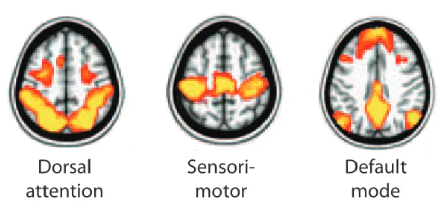
Figure 1: The dorsal attention, sensorimotor and default mode networks. Figure adapted from (31) .
task (1). Another explanation is that the spontaneous activation organizes neural activity and that the coordination is stronger between regions that commonly work together (1). The fluctuations could also serve as a dynamic prediction of the future with correlations occurring between regions that will probably be used together (1). However, no conclusive evidence exist for any of these hypotheses, and further investigation is needed.
Analysis of spontaneous BOLD data requires data-driven methods, such as seed-based correlation, hierarchical clustering, or ICA (see section 6). Independent com-ponent analysis has been widely used for analyzing both task-related and sponta-neous BOLD activity within neuronal networks (8; 11; 22–29).
In this work the focus is on three brain networks: the dorsal attention, the sensorimotor, and the default-mode networks illustrated in Figure 1. The sensori-motor network covers bilaterally the primary sensori-motor and somatosensory cortices as well as the supplementary motor area (SMA). In addition some other areas have been reported to covary with these areas, such as the thalamus and cerebellum (15– 20). The default mode network is distinct from the others in that its activation decreases during task performance (12; 13). It covers the posterior cingulate cortex (PCC) and precuneus, medial prefrontal cortex and bilateral inferior parietal cortex (23; 24;30). The fluctuations in this network have been suggested to be important for the processes during rest (12). However, the exact role of this network remains unclear.
Two sensory orienting systems, the ventral and dorsal attention networks, dy-namically interact and guide our attention. The dorsal attention network is involved in voluntary (top-down) processing of sensory information and links the selected sensory cues to appropriate motor responses. It includes the dorsal parietal cortex, particularly the intraparietal sulcus (IPS) and superior parietal lobule (SPL), and the junction of the precentral and superior frontal sulcus (frontal eye fields, FEFs) in each hemisphere (32). This network is activated by expectation of seeing a target in a particular location or with specific features, by the preparation of a response, or by short term memory of a visual scene (33).
environment, especially when unattended. The network is lateralized to the right hemisphere and includes the right temporal-parietal junction and the right ventral frontal cortex (32; 33). It is activated when targets appear in unexpected locations or when a target appears infrequently (33). The ventral system probably detects surprising events (stimulus-driven re-orienting) and disrupts the ongoing selection in the dorsal network which then shifts the attention to the novel target (34).
3
Naturalistic stimulation in fMRI
In human brain imaging, the interest has recently increased towards real-life-like stimulus settings. This section covers some of the work done in this field.
Traditional fMRI experiments use rather simple block designs, and the analysis is commonly done using the general-linear-model (GLM) analysis (see section6.2). Much of what is known about brain function by means of fMRI has been found out in this way. In the GLM approach, a hypothetical activation time course is constructed on the basis of the stimulus presentation. This time course is then compared with the measured data, and brain regions whose time courses match the modeled one in statistical sense are considered to be activated by the stimulus. Conventional fMRI experiments typically use rather simple stimuli in highly controlled conditions to reveal stimulus-dependent activations, which can be predicted and modeled. How-ever, in real life the environment is multimodal and constantly changing. If we want to know how our brains function in such situations, the stimulus settings in brain imaging should also be as naturalistic as possible. Quite recently fMRI experiments have started to utilize more naturalistic stimulation, such as movies (2; 3;5; 6;35– 39). Although movies are quite far from a real-life experience, they still mimic it well given the constraints of the experimental setup. On one hand, using naturalistic stimulation can reveal activity patterns that would not be found with traditional methods. On the other hand, the activations triggered by naturalistic stimulation should agree with the activations aroused by simple stimuli.
Because naturalistic stimuli often are highly unpredictable and multimodal, it may be difficult to use temporal covariates necessary for GLM analysis. The anal-ysis of fMRI data recorded during naturalistic stimulation therefore benefits from data-driven approaches that make no assumptions on activations triggered by the stimulus. The most widely used methods are seed-based correlation, ICA, and ISC (39). Data-based analyses have shown that human brain activity can be highly re-liable under naturalistic conditions (2; 3; 5–7; 35–39). The stimuli in these studies have included for example movies, audio books and music. For example, Bartels and Zeki (3) applied ICA and seed-based correlation to identify networks related to seeing, hearing and language processing. Correlations between directly connected regions increased during natural viewing while the correlation between unconnected regions decreased. In an earlier work, they used ICA to separate functionally con-nected brain networks from fMRI data collected during both free movie viewing and during a traditional block-design setup (2). Natural viewing activated more regions in a more distinct manner than did conventional stimuli.
4
Number of independent sources in fMRI data
In ICA, the number of components to be estimated has to be decided. How to determine the correct amount of independent sources in fMRI still remains an open question, although some attempts to address this issue have been recently taken. This section gives an overview of the research done concerning this problem.
Estimating too few ICA components leads to loss of information. McKeown et al. (29) concluded that compressing the data too much leads to loss of important information and thus it is better to estimate a large number of components. Many other studies have also concluded that a too low dimensionality causes ICA to mix various components (3; 9–11; 40). Ma et al. (41) detected RSNs with ICA and investigated the effect of the number of ICs on the results of ICA. They showed that a too low number of components affected the ICA results, but estimating too many components had no significant influence. An excessive reduction of the ICA dimen-sionality may be especially problematic when analyzing resting state fluctuations, because some of the sources are weak compared with noise (42).
On the other hand, estimating too many components causes splitting of the com-ponents (8–11). Li et al. (43) proposed a new method for order selection in ICA of fMRI data and showed that at too high dimensionalities the stability of the IC estimates decreases and the estimation of task related activations is degraded. Beck-mann and Smith (10) examined the dependency between the number of estimated components and the accuracy of the spatial maps and time courses of the estimated ICs. On one hand, estimating too few components led to loss of information and to suboptimal signal extraction, whereas estimating too many components caused overfitting and led to arbitrary splitting of the ICs due to unconstrained estimation. Smithet al. (8) investigated the splitting of RSNs, identified with ICA, using the massive BrainMap database including over 7000 functional maps collected during task conditions as well as resting state data from 36 subjects to calculate both 20-component and 70-20-component ICA compositions of both datasets. Similar brain networks in both datasets were found, which implies that the networks are active both in rest and during task performance. With the ICA-dimensionality of 70 the networks found in the 20-component composition split into smaller subnetworks of brain areas with slightly different function or into left- and right-sided subnetworks. Abou-Elseoud et al. (9) examined the effect of increasing the model order on IC’s characteristics of RSNs. Probabilistic group ICA (PICA) with ICASSO (see Section 6.5.6) was used for analyzing resting state fMRI data. At low dimension-alities, the signal sources merged into singular components, which were split into subcomponents with higher model orders. Also, some components emerged only at higher model orders whereas some did not split. The characteristics of the ICs,i.e. the volume and meanz-score, were significantly affected by the number of estimated components. The repeatability of the components decreased with increasing model order. Model orders around 70 were considered to offer a detailed and reliable eval-uation of the RSNs. Increasing the dimensionality further reduced reliability, but neither the meanz-score nor the volume showed any statistically significant changes.
5
Magnetic resonance imaging
This section gives a short overview of the basic principles of magnetic resonance imaging (MRI) as well as fMRI. The introduction starts from nuclear physics and proceeds step by step to image formation and different imaging techniques. The final part of the section introduces fMRI, a MRI technique to measure brain activity. This section is based on the textbooks of Huettelet al. (44), Buxton (45), and Liang and Lauterbur (46).
5.1
A short history of MRI
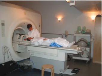
Magnetic resonance imaging utilizes high magnetic fields to produce images of bio-logical tissue. MRI is based on the phenomenon of nuclear magnetic resonance (NMR). The first NMR experiments were carried out in 1946 independently by two scientists and their research groups: Felix Bloch, working at Stanford University, and Edward Purcell from Harvard University. They found that certain nuclei placed in a magnetic field were able to absorb energy in the radiofrequency range of the electromagnetic spectrum and re-emit this energy. In 1970s, Raymond Damadian noticed that the NMR signal properties of cancerous tissue are different from that of healthy tissue. Paul Lauterbur introduced the idea of using field gradients in the magnetic field for NMR image formation and produced the first 2-D NMR image of test tubes containing water and heavy water in 1973. Peter Mansfield developed the echo-planar-imaging (EPI) technique for fast imaging. In the early 1980’s, the first magnetic resonance imaging scanners for humans became available. Figure 2shows the 3-T scanner used in this work located in Advanced Magnetic Imaging (AMI) Centre, Aalto University School of Science.
Figure 2: The 3T-MRI scanner (AMI Centre, Aalto University School of Science) used in this work.
5.2
Nuclear spins
The underlying mechanism of signal generation and detection in MRI occurs at the nuclear level. An atom consists of a nucleus, which includes protons and neutrons, and an electron shell. A fundamental property of nuclei is that they possess spin angular momentumJ~, whose magnitude is given by
J =~ps(s+ 1) s= 0,1
2,1, 3
2..., (1)
wheresis thespin quantum number, which takes either integer or half-integer values, and~thereduced Planck’s constant. Nuclei with odd mass number have half-integer spin, nuclei with even mass number and even charge number have zero spin, and nuclei with even mass number and odd charge number have integral spin. In MRI, a set of nuclei of same type present in the object being imaged is called a spin system. For example, the hydrogen protons in the human body form a spin system. Since hydrogen (H1) is the most abundant proton in the human body, it is the most commonly imaged nucleus in MRI. A hydrogen nucleus contains only one proton, so that it has a half-integer spin sH = 12.
Since the proton has a spin and carries a positive charge, it creates a magnetic field around it. The proton has amagnetic dipole moment ~µ, which is related to the spin angular momentum J~ by
~
µ=γ ~J , (2)
where γ is a nucleus specific physical constant called the gyromagnetic ratio. Al-though the magnitude of~µis known in any conditions, the direction of ~µis random in the absence of an external magnetic field. In an external magnetic field of strength B0, applied in the z-direction, the z-component ofµ can have values
µz =γms~ ms=−s,−s+ 1, ..., s , (3)
wheremsis themagnetic quantum number. For a hydrogen atom, the spin quantum
number is equal to 1
2 and thus hydrogen spin system is a spin-1
2 system. In a spin-1 2 system, the magnetic moment vector has two possible orientations: either parallel or anti-parallel to the external field.
In the external magnetic field B0, a spin experiences a torque that is equal to~ the rate of change of its angular momentumJ~
d ~J
dt =~µ×B~0. (4)
Because of the torque, the spin precesses about the z-axis with a stable angle with respect to the field. The angular frequency of this nuclear precession is
ω0 =γB0, (5)
which is known as the Larmor frequency. At 3T the Larmor frequency for a H1 nucleus is about 127,7 MHz.
5.3
Net magnetization
As noted earlier, in a spin-12 system, ~µcan either align parallel or antiparallel to the external field. Spins in different orientations have different energy states. For the spins that are aligned parallel with the external field the energy is
E↑ =−
1
2γ~B0 (6)
and for the spins aligned anti-parallel E↓ =
1
2γ~B0. (7)
Thus the energy states of the spins that are parallel to the external field are lower than those of the antiparallel spins. A spin is more likely to be in the lower energy state, so a small majority of the spins (at 3T an excess of 1∗10−6 spins) align parallel to the field. Although the population difference of the two energy states is very small, it creates a magnetization vector M~ from a spin system
~ M = Ns X n=1 ~ µn, (8)
where Ns is the number of spins. In a spin-12 system
µn,z =
+12γ~ if µn,z is parallel to the external field
−12γ~ if µn,z is anti-parallel to the external field , (9)
so that the magnetization vector is given by
~ M = ( N↑ X n=1 1 2γ~− N↓ X n=1 1 2γ~)~k= 1 2(N↑−N↓)γ~~k. (10) In equilibrium, the bulk magnetization vector points along the positive direction of the z-axis. The transverse component of M~ is zero at equilibrium because the precessing magnetic moments have random phases.
5.4
Radio-frequency excitation
The alignment of the spins with the external field does not as such lead to any measurable signal. To generate an NMR signal, a radio-frequency (RF) pulse is sent to the system. The RF pulse is an oscillating magnetic field perpendicular to B0. According to the Planck’s law, electromagnetic radiation of frequency ωRF carries
energy
ERF =~ωRF. (11)
To induce a transition of the spins from the lower energy state to the higher energy state, the radiation energy must be equal to the energy difference between these states
ERF =~ωRF = ∆E =γ~B0. (12) Or more simply
ωRF =ω0. (13)
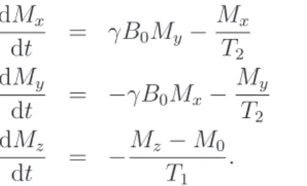
In thisresonance conditionspins absorb the energy from the RF pulse and flip from the low energy state to the high energy state so that the longitudal component of the net magnetization M0 decreases. In addition, the protons start to precess in phase, which establishes a transversal magnetization. This means that the RF pulse tippes the net magnetization vector to an angle θ with respect to the z-axis. The magnitude ofθ is proportional to the product of the duration and amplitude of the RF pulse and is called theflip angle(FA). The precessing net magnetization produces a time-varying magnetic field, which induces a current in a receiving coil located in the MRI scanner. Thus, a free induction decay (FID) signal can be measured. As the name implies, this signal decays in time because of spin relaxation. After the RF pulse is turned off, the individual spins start to loose their phase coherence and thus the transversal magnetization decreases (transverse relaxation). The time constant of this decay in a homogenous field is called T2. The spins also flip back to the lower energy state, which causes the longitudal magnetization to increase. This phenomenon is known as longitudal relaxation and its time constant is called T1, which is generally longer than T2. The combined process of precession and relaxation are described by the Bloch equations:
dMx dt = γB0My − Mx T2 (14) dMy dt = −γB0Mx− My T2 (15) dMz dt = − Mz−M0 T1 . (16)
Due to local magnetic field inhomogeneities, the FID signal actually decays faster than could be expected from a known T2. This enhanced decay is described by a time constant called T2∗, which plays a critical role in fMRI. It is defined as
1 T2∗ = 1 T2 + 1 T2′, (17)
where T2′ reflects the dephasing effect caused by field inhomogeneity. The T1, T2, and T2∗ values are tissue specific and are used as sources of contrast in MRI images.
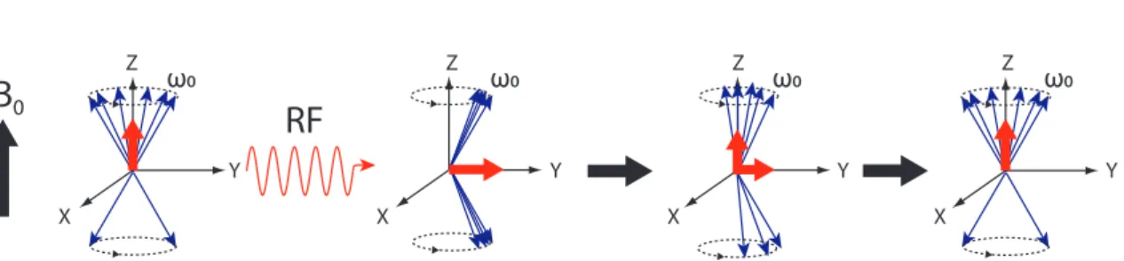
Figure3 shows the effect of the RF pulse and the relaxation of the spins.
5.5
Gradient fields
To image a three-dimensional object, three orthogonal gradient fields are superim-posed on the uniform external fieldB0. A gradient field is a spatially linearly varying~
B
0RF
X Y X Y ω0 ω0 X Y ω0 X Y ω0Figure 3: The majority of the protons align parallel to the external magnetic field
~
B0. The RF pulse flips some of the protons to the higher energy state (antiparallel
to the external field), which causes the longitudal magnetization (red arrow) to decrease (with a 90o pulse it goes to zero, as in the figure). The protons start to
precess in phase, which causes a transversal magnetization. After the RF pulse, the protons start to lose their phase coherence (transversal magnetization decays) and flip back to the lower energy state (longitudal magnetization recovers). Note that the figure is illustrative and the number of spins in the two energy states is not proportional to the true population difference.
field produced by gradient coils in the scanner. The variations caused by the gradi-ent fields are small compared with the main magnetic field. Since MR images are sampled in three dimensions, the basic sampling units of MRI are three-dimensional volume elements called voxels.
The slice selection gradientis applied in the same direction as the uniform mag-netic field. It causes the resonance frequency of the spins to vary linearly along the z-axis. This gradient field is applied while an RF pulse containing only a narrow band of frequencies centered at the desired ω0 is sent. In this way it is possible to excite spins in a certain slice, i.e. those spins that are in resonance with the RF pulse. Slice thickness can be altered by changing the bandwidth of the RF pulse or by modifying the steepness of the gradient.
To determine a specific voxel in the slice from which the signal is coming, two additional gradients are used. The frequency-encoding gradient is in a typical MR-imaging sequence applied after the radio frequency pulse and it results in different precession speeds along the x-axis. The phase-encoding gradient is turned on for a short time after the RF pulse and it is perpendicular to the frequency encoding gradient. When the gradient field is applied, the protons start to precess at different frequencies. When the gradient is then turned off again, the protons go back to their former precession frequencies, but now they have different phases. The result is a mixture of signals with different frequencies and phases. The frequency and phase information are collected in a so called k-space(47;48). The spatial MR image can then be reconstructed from the measured data using the Fourier transform.
5.6
Pulse sequences and image contrast
Because the signal decays in time, a new RF pulse is applied to trigger a new signal. The time between successive excitation pulses is called the repetition time (TR). Generally, the FID signal is not measured, but an echo of the original signal is
RF
1 ... n
Slice selection Phase encoding Frequency encoding RF DAQ 1 ... n 180o 90o 90o TE TR a) b) DAQ TR TE
Figure 4: a) A spin-echo pulse sequence and b) a gradient-echo pulse sequence. DAQ = data aquisition.
created occurring at a time TE, the echo time. In a spin-echo sequence this is done by sending in a second RF pulse after a delay of TE/2. Commonly a 180o pulse called the refocusing pulse is used, because it creates the strongest echo. After the original 90o pulse, the spins start to lose their phase coherence, because they precess at slighly different rates. The spins that precess faster get ahead of the slower ones. The 180o pulse flips the spins so that the phase acquired by each spin is converted into a negative phase. Now, the faster-precessing spins are behind the slower ones. At t =TE, the faster-precessing spins have caught up with the slower ones and the spins are back in phase and create an echo. A gradient-echo sequence uses gradient fields instead of a refocusing pulse to generate the signal echo. In this sequence a negative field gradient is turned on after the RF pulse to dephase the spins, which are then rephased by a subsequent positive gradient. Gradient-echo sequences typically use small flip angles (<90o) and thus the TR can be reduced, which in turn reduces the scanning time. Figure 4illustrates these two types of pulse sequences.
If TR is much longer than T1, the spins recover to equilibrium after each pulse and the signals after succeeding pulses are equally strong. As the TR is shortened, the signal generated by the second RF pulse becomes weaker, since the spins have not relaxed completely. Because the T1 values are tissue-specific, the spins in some
S I R L A P S I L R P A
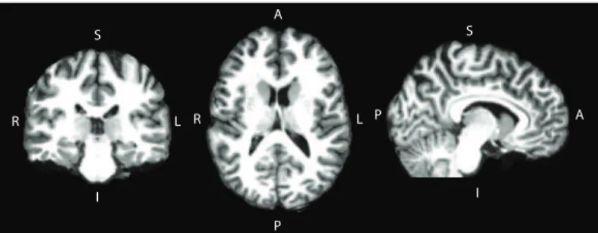
Figure 5: T1-weighted skull-stripped MR image from one of the participants of this study showing coronal, axial and sagittal slices. The abbreviations refer to the orientation of the figure: right (R), left (L), superior (S), inferior (I), anterior (A), posterior (P).
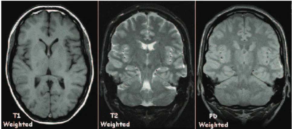
Figure 6: Example of T1-, T2- and a PD-weighted images. The cerebrospinal fluid appears black in T1-weighted images and white in T2-weighted images. PD-weighted images show only little contrast between tissue types. Figure adapted from
http: // en. wikibooks. org/ wiki/ File: T1t2PD. jpg.
tissues have recovered more than in others and give thus a stronger signal. This creates a contrast between different tissue types, and the resulting image is called T1-weighted. Fat appears bright and water dark in T1-weighted images. Figure 5 shows an example of T1-weighted MRI images in three orthogonal slice orientations: the coronal, axial and sagittal slices. Figure 6 (left) compares a T1-weighted image with images acquired with other contrast weightening.
The signal received is proportional to the net magnetization M0, which in turn depends on the amount of protons in the tissue. For the tissues in the body, proton density (PD) and T1 are positively correlated. This conflicts with the T1-contrast, because a tissue with high proton density has a greater net magnetization and therefore a larger signal than a tissue with low proton density. On the other hand, long T1 tends to make the same tissue darker because there is less recovery at long T1. A proton-density-weightedimage can be produced if the TR is long enough so that the spins have had time to relax in all tissue types. With a small flip angle the recovery is faster and the longitudal magnetization is hardly affected by the RF pulse; the sensitivity to differences in T1 is greatly reduced. Figure 6 (right) shows an example of a PD-weighted image. PD-weighted images show less contrast between tissue types than T1-weighted images.
TE is an important parameter for T2-weightedimages. With TE<T2, transver-sal decay is small and the T2 contrast is weak. If the TE is too long, nearly all transversal magnetization will be lost and thus there is no T2 contrast. However, with TE ≈ T2, the signal is strongly sensitive to the local T2, and T2 contrast can be maximized. T2-weighted images provide maximal signal from fluid-filled regions, as is seen in Figure 6 (middle).
T2∗-weighted images are sensitive to the relative concentration of deoxygenated
haemoglobin in the blood, which changes according to the metabolic demand of active neurons. T2∗-contrast is best achieved with gradient echo pulse sequences
with long TR and medium TE. Spin-echo sequences have reduced T2∗-sensitivity,
basis for BOLD-contrast fMRI, described in more detail in Section 5.7.
5.7
Functional magnetic resonance imaging
5.7.1 The BOLD effectFMRI provides information on brain physiology. Theblood oxygenation level depen-dent (BOLD) effect, discovered by Ogawa and coworkers in 1990 (49), is the most widely used source of contrast in fMRI. It arises because of two distinct phenomena: the different magnetic properties of oxygenated and deoxygenated heamoglobin and changes in blood flow.
Neurons in the brain continuously consume glucose and oxygen (O2), which are supplied by the cerebral blood flow (CBF). In the blood, oxygen is bound to haemoglobin. Oxygenated haemoglobin is diamagnetic whereas deoxygenated haemoglobin is paramagnetic. Therefore, changes in the relative concentration of oxygenated vs. deoxygenated haemolobin result in changes in the BOLD signal, which is stronger when less deoxygenated haemoglobin is present. In an active brain area, the cerebral metabolic rate of O2 consumption (CMRO2) increases and haemoglobin becomes deoxygenated. At the same time, more blood is brought to the active site. Because the blood flow increases much more than the CMRO2, the amount of oxyhaemoglobin in the blood is increased and the relative concentration of deoxygenated haemoglobin is decreased, which results in a stronger MR signal.
BOLD effects are commonly measured using T2∗-contrast. The presence of
de-oxygenated hemoglobin makes the magnetic field stronger in the red blood cells than in the surrounding plasma, which creates field inhomogeneities that shorten the T2∗.
In an active brain area the relative concentration of deoxygenated hemoglobin is de-creased and thus the field inhomogeneities are reduced. T2∗ becomes longer and the
signal is increased in a T2∗-weighted image.
5.7.2 Echo planar imaging
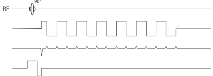
To detect brain activity, images have to be acquired very rapidly, approximately at the same rate as the physiological changes happen. One approach to reduce the scanning time is to collect data corresponding to more than one phase-encoding step from each excitation. Figure7shows the most popular sequence suited for fast
90o
RF
. . .
. . .
0 5 10 15 20 25 30 Time (s) −0.02 0 0.02 0.04 0.06 0.08 0.1 A . U .
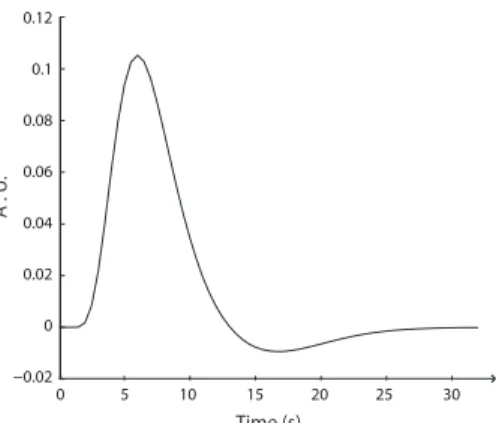
Figure 8: The shape of a typical haemodynamic response to a single short-duration event.
imaging, theecho planar imaging(EPI) sequence, originally developed by Mansfield in 1977 (50). Here, the gradients oscillate so rapidly that all the phase-encoding steps required for an image can be measured after a single excitation. Thus the whole k-space is filled after each RF pulse.
Fast scanning enables the detection of functional changes in the brain, but it impairs the spatial resolution. EPI images have low signal-to-noise ratio and the contrast between different tissues is poor. Therefore, high resolution structural MRI images are often acquired so that statistical maps of the functional images can be superimposed on them to better pinpoint the activation sites.
5.7.3 The haemodynamic response
The change in the dynamics of the BOLD signal triggered by neuronal activity is called the haemodynamic response (HDR). The shape of the HDR can vary in different brain areas and between individuals (51). The first observable HDR changes occur with a 1–2 s lag with respect to the neuronal events that initiate it. The HDR is typically modeled with a canonical haemodynamic response function (HRF), shown in Figure 8 to a single short-duration event (occurring at t = 0) and modeled as a gamma-variate function.
An initial negative dip may precede the response (52; 53) and it has been at-tributed to a transient increase in the amount of deoxygenated blood. The initial dip is however often not separately modeled. After a short latency the signal rises, because more oxygen is brought to the area than is extracted by the neurons. The signal reaches its peak at about 5 s. If the stimulus lasts for a longer time, the peak is extended to a plateau. About 6 seconds after the peak, the signal decreases below baseline. The poststimulus undershoot results from faster decrease of blood flow than blood volume after the neuronal activity has returned to baseline. Thus, the relative amount of deoxygenated blood increases and the fMRI signal is reduced below baseline levels. When the blood volume slowly returns to normal level, the signal rises back to baseline.
6
Analysis of fMRI data
This section focuses on the analysis of fMRI data. First, the typical image prepro-cessing necessary prior statistical analysis is explained. Then the most widely used method for determining brain activation in fMRI, the general-linear-model (GLM) based analysis, is introduced. Finally, the data-driven methods used in this work are presented, concentrating mainly on independent component analysis.
6.1
Pre-processing of images
The BOLD images are noisy and suffer from several types of artifacts, such as head movements. In addition, the images acquired from different subjects are not directly suitable for group analysis. Thus, careful preprocessing is necessary before the analysis. This section explains the main pre-processing steps implemented in the SPM8 software, which was used in this work.
6.1.1 Slice-timing correction
Because the slices in a volume are acquired at slightly different times, the measured signal has a sampling delay in each slice. To correct for this error, the data are often retimed. This is usually done by temporal interpolation, which uses information from nearby time points to estimate the amplitude of the signal at the onset of the TR. No retiming was however applied to the data of this work due to a quite modest TR (2.015 s).
6.1.2 Realignment
Head motion is probably the most damaging artifact in fMRI. If the head moves during scanning, the signal from a given voxel will be from different parts of the brain in succeeding images. Head-motion-related artifacts are corrected by realign-ingthe images. The images are coregistered to a single reference volume using arigid body transformation, which assumes that the shape of the head does not change and corrects for rotations and translations along the x-, y- and z-axes. In spatial regis-tration, the parameters that either maximise or minimize some objective function, such as sum of squared differences, are estimated and then applied to the images. 6.1.3 Coregistration
The functional images are coregistered to the structural images from the same sub-ject to facilitate the mapping of low-contrast functional data on high-resolution and high-contrast anatomical images. The coregistration of functional images to struc-tural ones differs from motion correction in two ways. First, the head may not be the same shape in the structural and functional images. Thus, instead of a rigid-body transformation, non-linear transformations are used. Second, the intensity values are different in these two types of images. Therefore, simple cost functions, such as
the sum of squared differences, are not appropriate. For example, mutual informa-tion can be used as a cost function in functional-structural image coregistration. 6.1.4 Spatial normalization
The shape and size of the head varies remarkably across individuals. For group anal-ysis or for averaging effects across subjects, the brains in the images arenormalized into a standard coordinate system, such as the Talairach space or the Montreal Neurological Institute (MNI) space. In SPM, the procedure has two steps. The first step is a 12-parameter affine transformation to match the size and position of the images. The second step is a non-linear affine transformation, which is modeled by linear combinations of three-dimensional smooth discrete cosine basis functions. The parameters of this non-linear transformation can be found for example within a Bayesian framework, which estimates the most likely regional deformations and then combines them with the global transformations.
6.1.5 Spatial smoothing
Spatial smoothing reduces the high-frequency spatial components and ”blurs” the images. The smoothing is commonly done by spatially low pass filtering the data with a Gaussian filter. Smoothing improves the signal-to-noise ratio and the validity of statistical analysis by making the error distribution more normal. It also decreases the differences across subjects in the sites of brain activations.
6.2
The general linear model
To examine real activations in the low-resolution fMRI images, the data are sub-jected to statistical analysis. The most common way is to use the GLM-based analysis. To find brain areas most affected by the stimulus, a reference time course is constructed by convolving the stimulation time course with a haemodynamic re-sponse function. This reference time course is then inserted into the GLM as a covariate. The basic idea is that the observed datax can be modeled as a weighted sum of several covariates gi:
x=β1g1+β2g2+...+βngn+ǫ, (18)
whereβi are the parameter weights, which tell how much each covariate contributes
to the overall data, and ǫ is the error term. For different conditions, a time course can be modeled for each one separately. Known sources of variability, such as head movement or respiration, can also be added as nuisance covariates to improve the validity of the GLM. After the model has been constructed, the weights are approx-imated by least-squares estimation. The statistical significance of the estapprox-imated weights can be tested with t-statistics. The analysis can be extended to group level by inserting the individual contrast images into a random-effects analysis to reveal brain areas that are statistically significantly activated in the whole group of subjects.
The use of the GLM requires that the responses can be predicted and a reference time course can be formed. If we want to reveal brain activations during more naturalistic conditions, where the stimulus is multimodal and highly unpredictable, GLM is no longer feasible for the analysis. Purely data-driven approaches, such as inter-subject correlation or independent component analysis, need no a priori models of the stimulus-related activations, and are thus sometimes more suitable for analyzing fMRI data acquired during naturalistic stimulus presentation.
6.3
Inter-subject correlation
Inter-subject correlation analysis, proposed by Hasson et al (39), is a data-driven model-free approach for analyzing fMRI data. With ISC it is possible to reveal brain areas whose temporal behaviour is similar across subjects during continuous and complex stimulus presentation, such as watching movies. ISC uses the signal of one subject to model the signal in the corresponding voxels for other subjects by correlating the time series. The signals are correlated voxel by voxel for each subject pair. The correlation maps for all subject pairs are then subjected for group-analysis by testing for significance, for example with at-test. ISC has been shown to segregate e.g. the extrinsic, stimulus-driven brain networks from the intrinsic, spontaneous BOLD-signal fluctuations (35; 54).
6.4
Seed-based correlation
In seed-based correlation, the measured signal from a pre-defined seed point is cor-related with signals from other voxels of the brain to reveal brain areas that are functionally connected with this seed point. The analysis can be extended to group level by subjecting the individual connectivity maps for statistical analysis.
6.5
Independent component analysis
This section is mostly based on the tutorial paper on ICA by Hyv¨arinenet al. (55). 6.5.1 Motivation
Let’s start with a popular simple example to describe what ICA is. Imagine two people speaking in a room and two microphones recording their speech. The signals recorded with the microphones are mixtures of these two speech signals. With ICA, it is possible to estimate the original source signals—the two speech signals—from the mixture signals recorded with the microphones. The mixing of the two speech signals depends on many factors, such as the locations of the microphones and the acoustic properties of the environment. If this mixing would be known, separating the two signals would be easy and could be done by classical methods. However, both the mixing and the original source signals are often unknown and we only have the recorded signals, which makes the problem difficult. One approach for solving the problem is to use some information about the statistical properties of the source
(a)
(b)
(c)
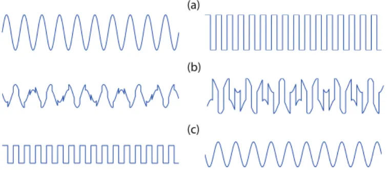
Figure 9: A simple example on how ICA works. (a) The original signals, (b) two mixed observations of the source signals, and (c) the source signals estimated with ICA. These independent components match very well the original signals, with only small differences in scales and signs. FastICA on own simulated data.
signals to estimate the mixing. ICA is based on the assumption that the source signals are statistically independent. This assumption is often tenable, and actually does not have to hold exactly for ICA to work (55). ICA can be implemented by many algorithms, such as Infomax (28) and FastICA (56). Figure 9 shows a simple example on how ICA separates two source signals from two mixed signals. In fMRI, the mixed signals are the acquired BOLD signals and the source signals are temporally/spatially independent brain networks.
6.5.2 Definition of ICA
ICA is an approach for solving the blind source-separation problem, which is the problem of separating the original signals from a set of mixed signals without in-formation (or with very little inin-formation) about the source signals or the mixing process. The ICA model is formulated as a generative linear latent-variables model. Latent means that the independent components cannot be directly observed. Gen-erative means that the model describes how well the observed data are generated by a process of mixing the components. When the data are represented by a random vector x and the independent components by s, the mixing can be expressed in matrix form as
x=As, (19)
where A includes the mixing weights ai and is therefore called the mixing matrix.
The ICA model assumes that the components are statistically independent and have non-gaussian distributions. In practice, the ICs are obtained by estimating the inverse matrix W=A−1
6.5.3 Measures of non-gaussianity
ICA estimates the independent components by maximizing an objective function, which measures nongaussianity. Measures of nongaussianity are for example kurtosis and negentropy. Kurtosis is estimated by using the fourth-order statistical moment and is defined as
kurt(s) =Es4 −3Es2 2, (21)
whereE{·} stands for the expectation value. Kurtosis is simple to compute, but it is very sensitive to outliers (57).
Another measure of nongaussianity is negentropy, which is based on the informa-tiontheoretic quantity of entropyH, which in turn is a measure of uncertainty. The entropy of a random variable is larger than that of a structured and predictable one. Since gaussian variables have the largest entropy among all random variables with equal variance (58), minimizing entropy corresponds to maximizing nongaussianity. Negentropy can be considered as negative entropy, and it is defined as
J(s) =H(sgauss)−H(s), (22)
where sgauss is a gaussian random variable with the same covariance matrix as s.
Negentropy is zero for gaussian variables and always non-negative. Calculating the negentropy according to its definition is computationally difficult and in practice approximations are used.
Another approach for ICA estimation is to minimize mutual information. Mutual informationIgives the amount of information shared between random variables and is defined as
I(s1,s2, ...) =X
i
(H(si)−H(s)). (23)
Mutual information is closely related to negentropy. ICA estimation by minimizing mutual information is equivalent to maximizing the sum of nongaussianities of the estimates.
Independent components can be estimated for example with the algorithm called FastICA (56), which was used in this work. It uses negentropy as an objective function and a fixed point optimization scheme based on Newton-iteration.
6.5.4 Preprocessing for ICA and order estimation
Before estimating the independent components, some further preprocessing has to be done. The observed data are centered (made zero mean) and whitened (uncor-related and normalized). Whitening can be done for example with principal com-ponent analysis (PCA) (59). PCA transforms the possibly correlated variables into uncorrelated variables calledprincipal components. The components are ordered so that the first principal component explains most of the variance of the data. Each succeeding component accounts for as much of the remaining variability as possible.
One way of finding the principal components is to use the eigenvalue decomposition (EVD) of the covariance matrix EexxeT of the data:
EexexT =EDET, (24)
whereE is the orthogonal matrix of eigenvectors of the covariance matrix and D is the diagonal matrix of its eigenvalues. The data can now be whitened
e
x=ED−1/2ETx. (25)
Whitening transforms the mixing matrix A into a new one, A, and the whitenede ICA model can be written as
e
x=ED−1/2ETAs=As.e (26)
Since Ae is orthogonal, whitening reduces the amount of parameters to be es-timated. The dimension of the data can be reduced by leaving out the weakest principal components. This often improves the signal-to-noise ratio and reduces the risk of overfitting, which is sometimes observed in ICA (56). The right number of true components is not known, but several methods exist to estimate it. The mini-mum description length (MDL) criterion, which was used in this work, is based on the minimum code length (60). The MDL criterion for order selection is
EM DL(k) =−L(x|Θk) +
1
2G(Θk) logN, (27) whereL(x|Θk) is the maximum log-likelihood of the observations,i.e. the measured
signalsx, based on model parameters Θk of thekth order andG(Θk) is the penalty
term for model complexity given by the total number of free parameters in Θk and
N is the number of samples (in case of fMRI images, the samples are the voxels). The maximum log-likelihood is given by (43)
L(x|Θk) = N 2 log QT i=k+1λ 1/(T−k) i 1 T−k PT i=k+1λi T−k , (28)
where T is the original dimension of the multivariate data and λi is the ith
eigen-value of the covariance matrix EexxeT of the measured data. The number of free
parameters is given by (43)
G(Θk) = 1 +T k−
1
2k(k−1). (29)
Estimating too few components leads to loss of information. On the other hand, overestimation could result in splitting of the informative components and in spuri-ous components due to unconstrained estimation and factorization that will overfit the data (10).
6.5.5 Ambiguities of ICA
ICA has two main ambiguities. First, the signs and scales of the sources cannot be identified. Second, the ICs do not appear in any specific order. What is more, all ICA algorithms converge to slightly different results in separate runs.
6.5.6 ICASSO
ICASSO (61) is an algorithm for investigating the reliability of the components. ICASSO runs ICA several times with different initial values and/or with differently bootstrapped data sets. The estimated components are clustered according to a similarity measure, such as absolute correlation. The stability index of the ICA-estimate clusters is computed as the difference between intra-cluster similarities and average extra-cluster similarities, and it provides a quantative estimate of the compactness of the clusters. If the stability index is close to unity, ICA estimation is stable and consistent, meaning that similar components are estimated at every run of the algorithm. The tighter the cluster a component belongs to is, the more reliable the IC is. The most unreliable components do not belong to any cluster. The cluster centers represent the ideal components. ICASSO was used in this work, since it is inbuilt in the group-ICA toolbox (62) that was used for ICA analysis. However, also other methods for estimating the consistency of ICs exist (63; 64). 6.5.7 Application of ICA to fMRI data
ICA is well suited for analyzing fMRI data, since both activity-related signals and noise match the assumptions and limitations of ICA (29). One advantage of us-ing ICA in fMRI data analysis is that it separates some of the noise sources as independent components (29; 65).
Spatial ICA is typically used in the analysis of fMRI data. Spatial ICA finds systematically non-overlapping brain networks without constraining the temporal domain. In the spatial model, the rows of the data matrix contain the images and the columns are the voxels. The rows ofSare the spatially independent components. The columns of the mixing matrix A contain the weights, i.e. the time courses of the spatial ICs.
6.5.8 Group ICA
ICA analysis can be extended to group level. Calhounet al. (62) proposed a method for performing group ICA, which was also used in this work. The first step is data reduction, which can be done in either two or three stages. First the dimension of each subject’s functional data is reduced. Then, the data from all subjects are concatenated together and the dimension of this aggregate data set is reduced. The reduced aggregate data matrixX is then (62)
X=G−1 F−1 1 X1 . . F−1 MXM (30)
where M is the number of subjects andG−1 andF−1
i are the reducing matrices from
PCA for the concatenated data set and for subjecti, respectively. Xi represents the
original data matrix from subject i, in which one row contains one volume of fMRI data. Alternatively, the subjects can be divided into groups of which the dimension is decreased before the final data reduction. The next step is to apply ICA to the reduced data set. The mixing matrix can further be partitioned according to individuals and the ICA model can then be written as
G1 . . GM AˆˆS = F−11X1 . . F−M1XM , (31)
whereAˆ is the mixing matrix for the group data andSˆ is the component map. The individual subject components ˆSi can be also reconstructed utilizing the matrices
G and F:
ˆ
Si = (GiA)ˆ −1F−i 1Xi. (32)
The ICs of individual subjects can be used for calculating the mean components and for t-statistics. Both the group components and the individual subject components can be scaled for visualization using percent signal change orz-scores.
7
Materials and methods
7.1
Subjects
Twenty two healthy volunteers (9 females, 6 males, mean age 24 years, range 19– 49 years) participated in the study after written informed consent. The study had prior approval by the Ethics Committee of Helsinki and Uusimaa Hospital District. Altogether, the data from 7 subjects were rejected because of technical problems, drowsiness of the subject or excessive head movements; thus, the following analyses are based on data of 15 subjects.
7.2
Stimuli
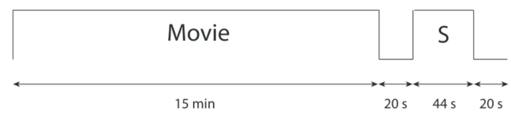
During fMRI scanning, the subjects viewed a 15-min silent film (At Land by Maya Deren, 1944). The film was followed by a 44-s long compressed version of the film. This summarization consisted of 22 2-s episodes from the film selected by means of an automatic video summarization algorithm (66). The algorithm analyzed low level features and the selection was additionally weighted by face and movement detection. The summarization was preceded and followed by 20-s resting periods, during which the subjects were asked to fixate on a cross. Otherwise, the subjects’ task was simply to watch the movie and the summarization. Figure10illustrates the order and durations of the stimuli. The stimuli were delivered using the Presentation software (version 0.81, http://www.neurobehavioralsystems.com). Videos were projected (projector Vista X3 REV Q, Christie Digital Systems, Canada, Inc.) to a transparent screen placed behind the subjects, which the subjects viewed via a mirror.
7.3
Data acquisition
The fMRI images were acquired with a Sigma VH/I 3.0 T MRI scanner (General Electric, Milwaukee, WI, USA). Functional images were obtained using gradient echo-planar-imaging sequence with following parameters: TR 2.015 s, TE 32 ms,
Movie
S
15 min 20 s 44 s 20 s
Figure 10: The order of stimuli. The 15 min long movie was followed by a 44-s summarization (S) of the movie.
FA 75o, 34 oblique axial slices, slice thickness 4 mm, matrix 64×64, voxel size 3×3×3 mm, field of view (FOV) 22 cm. Altogether 485 volumes were collected. These volumes included 4 dummy scans (the first scans that were acquired to ensure that a spin system was in a steady state before data collection), which were removed from further analysis. Structural images were scanned with 3-D T1 spoiled gradient imaging, matrix 256 x 256, TR 10 ms, TE 3 s, flip angle 15o, preparation time 300 ms, FOV 25.6 cm, slice thickness 1 mm, number of excitations 1. Movements of the subject’s right eye were followed with SMI MEye Track long-range eye tracking sys-tem (Sensomotoric Instruments GmbH, Germany), based on video-oculography and the dark pupil-corneal reflection method. The eye-tracking data were not utilized in this thesis.
7.4
Pre-processing
The fMRI data were preprocessed using SPM8 software (http://www.fil.ion.ucl. ac.uk/spm/software/spm8/), including realignment, co-registration, normalization into MNI space and smoothing with a 6-mm (full-width half maximum) Gaussian filter. Before normalization, the images were skull-stripped using the FreeSurfer software (http://surfer.nmr.mgh.harvard.edu/).
7.5
ICA
The IC analysis was performed with the GIFT software (version v2.0d, http:// icatb.sourceforge.net/groupica.htm) for group-ICA. The number of sources was estimated to be 70 using the minimum description length algorithm inbuilt in GIFT. Twenty five, 40 and 70 ICs were calculated with the Fast ICA algorithm. ICASSO analysis was done to confirm the reliability of the components. Three ICs, representing the sensorimotor, dorsal attention and default-mode networks, were selected by visual inspection from the 25-component decomposition. From the decompositions of 40 and 70 components, respectively, ICs were selected by visual inspection so that they together resembled the spatial maps of the selected ICs from the 25 component decomposition. The selection was facilitated by spatially correlating the unthresholded spatial maps with the three 25-component maps. Most of the selected subcomponents belonged to the eight ICs with highest correlation coefficients. The correlations between the time courses of the selected components were computed.