Ž .
Energy Economics 23 2001 141᎐151
The impact of mitigating CO emissions on
2Taiwan’s economy
Tser-yieth Chen
UMing-Chuan Uni¨ersity, Institute of Management Science No. 250, Chung-Shan North Road, Section 5, Taipei 111, Taiwan, PR China
Abstract
In this paper, a computationally multi-objective programming approach and a Leontief inter-industry model are used to investigate the impact of mitigating CO emissions on2
Taiwan’s economy. The estimated result shows that Taiwan’s GDP will drop 34% off the targeted GDP growth rate for the year 2000 and Taiwan’s economy will be seriously weakened if annual CO emissions are stabilized at the 1990 level. When Taiwan maintains2
CO emissions at 128% of the 1990 level, then Taiwan’s economy will be able to show a2
5.37% average annual growth rate up to year 2000; a 157% CO emission level would mean2
a 5.92% annual GDP growth rate; and a 213% CO emission level for a 6.85% annual GDP2
growth rate. In addition, policy implications are presented in order to provide policy makers in economic planning.䊚2001 Elsevier Science B.V. All rights reserved.
JEL classifications:Q48; Q40
Keywords:Greenhouse effect; Interindustry analysis; Multi-objective programming
1. Introduction
There is growing concern that in increasing accumulation of carbon dioxide in the atmosphere is leading to undesirable changes in global climate, such as the greenhouse effect. This has resulted in proposals to set physical targets for reducing emissions of CO . The Framework Convention on Climate Change2
ŽFCCC was signed in Rio de Janeiro by more than 150 countries to promote.
U
Corresponding author. Tel.:q886-2-2882-4564; fax:q886-2-2739-0533.
Ž .
E-mail address:[email protected] T. Chen .
0140-9883r01r$ - see front matter䊚2001 Elsevier Science B.V. All rights reserved. Ž .
international cooperation for achieving such reductions in June 1992. These countries officially addressed an international target to stabilize CO emissions at2 the 1990 level by the year 2000 among the 36 Annex I countries.1 The second
Ž .
Assessment Report of the Intergovernmental Panel on Climate Change IPCC , approved in December 1995. It acknowledge that global CO emissions should be2 less than 50% of current levels in order to stabilize CO atmospheric concentra-2 tions, and that the Annex I countries should make an effort to limit and reduce their emissions within a given time frame. Furthermore, a legal grounding was
Ž .
agreed upon at the convention of parties COP III meeting in Kyoto, Japan, in December 1997, to acknowledge that global CO gas emissions should be reduced2
by 5.2% of 1990 levels among 38 industrialized countries. COP III also demanded that all developing countries should be included in CO emission reduction efforts;2 this will be discussed in the next COP IV.
Basically, Taiwan must pay close attention to the issue of global environmental change because the international trade plays a critical role on Taiwan’s economy. By the end of 1996, total CO emissions in Taiwan were 1712 =106 tons. Projected
CO emissions in 2000 will reach 2362 =106 tons, which is 203% of the 1990 level
Ž116=10 tons . From 1990 to 2000, the average growth rate of CO emissions will6 . 2
be 7.1%. This Taiwan government may initiate relevant policy actions in the foreseeable future to fulfill its global responsibility in reducing production of CO ,2 which contributes to the greenhouse effect. With this in mind, it is important to understand the current progress of advanced countries in implementing such policy actions and to simulate the impact of domestic measures to reduce greenhouse CO2 emissions on Taiwan’s economy.
In this paper, we use a multi-objective programming to estimate the trade-off between GDP and CO emissions in Taiwan. In order to achieve this objective,2
relevant literature is first reviewed. A multi-objective programming coupled with an input᎐output model is constructed to evaluate the economic impact of reducing CO emissions on the Taiwan economy as a whole. Empirical data are collected2 and various options for mitigating industrial CO emissions are simulated. Based2 on the simulation, policy implications are discussed and some suggested for the future research are recommended.
2. Literature review
Ž .
As to the previous studies, Loucks 1975 addressed multi-objective programming within resource utilization and economic development decisions, with each
ob-1
( )
T. ChenrEnergy Economics 23 2001 141᎐151 143
Ž .
jective being a trade-off itself. Hafkamp and Nijkamp 1982 presented a multi-objective programming approach and applied it to the issue of integrated resource planning. They argued that a single-objective model cannot assess social welfare
Ž .
changes accurately. Nijkamp 1986 employed multi-objective approach to evaluate
Ž .
the policy impact of resource allocation. Nordhous 1992 and Morrison and Brink
Ž1993 conducted two surveys to present the economic costs of mitigating climate.
change.
Among the programming model on the mitigation of CO emissions, four papers2
Ž .
are reviewed here. Manne and Richels 1991 established a Global 2100 model, which is a programming analysis, to evaluate the costs and benefits of controlling
Ž .
CO2 emissions for the US. Rose and Steven 1993 presented a non-linear programming model to simulate the net welfare changes of various strategies for
Ž .
the mitigation of CO emissions for eight countries. Fells and Woolhouse 19942 provided an optimization model to estimate the impact of mitigating CO emis-2
Ž .
sions on economic growth in the UK. Finally, Rose 1995 provided a linear-pro-gramming model to evaluate reduction in GDP resulting from five proposed CO2 emissions mitigation programs in Mainland China.
3. The multi-objective programming model
In this section, a multi-objective programming combined with an input-output model is employed to determine the trade-off between GDP growth and CO2 emissions on Taiwan’s economy. There are three reasons. First, the multi-objective approach is superior to the single-objective method, in that it focuses on the range of choices associated with a decision. The decision-maker can judge the relative values of objectives and find the ‘best’ possible values under the given conditions
ŽZeleny, 1982 . Second, multi-objective programming emphasizes resource alloca-.
tion, i.e. it determines what the economy should ideally be like. Multi-objective analysis can derive trade-off between economic and environmental objectives subject to constraints. Third, the multi-objective approach can avoid some issues of econometric modeling, such as heteroscedasticity, autocorrelation, multicollinear-ity, etc. The model for the problem to be solved in the present paper is stated as:
Ž . Ž Ž . Ž .. Ž .
MaxUs GDP,CO emissions2 s G X ,yC X s VX,yCX
subject to
d Ž . d
F1994F 1yAqM XsF2000
where GDP presents gross domestic product. X represents the n=1 vector of
sector output, i.e. the dependent variables of this model.V is the 1=n vector of direct income coefficients, i.e. the ratio of sectional value-added to total sales for each sector, and n represents 33 industrial sectors. C is the 1=n vector of CO2 emission coefficients, i.e. the ratio of total CO emissions of energy in each sector.2
Fd2000 and Fd1994 are, respectively, the n=1 vectors of the 2000 and 1994 levels of final demand. I is the n=n unit matrix, A is the n=n matrix of technical coefficients and M represents the n=n diagonal matrix of import coefficients. Furthermore, Xu and XL present the n=1 vectors of the projected upper and lower limits, respectively, of the production level of each sector in the year 2000. L
represents the 2=n matrix of labor input coefficients, i.e. the ratio of labor
Ž
employed to total sales for each sector two types of labor were measured, i.e.
.
technical and non-technical labor , and Lmax is the 2=1 vector of the two-types of
labor employed.W is the 1=n vector of water utilization coefficients, is the ratio of water utilization to total water supply for each sector, and Wmax means the maximum resource limit of the water supply.
Ž . Ž .
In this model, G X has the objective of maximizing GDP and C X has the
Ž .
objective of minimizing CO emissions.2 C X is multiplied by y1 because CO2 emissions are to be minimized. The first constraint set is derived from the relationship XyAXqMsF, which indicates that the sum of domestic output
Ž .
and importation in each industry sector which is total supply must be equal to the
Ž
intermediate requirement of other sectors and the final demand sector which is
.
total demand . Also, the level of each final demand sector in year 2000 cannot be less than in the year 1994. This is a general equilibrium restriction. The second and third constraint sets limit each sector to a specified upper bound of capacity expansion and to a lower bound of depressed scale. The last two constraints are the labor and water supply conditions, respectively.
4. Empirical results
The data in the model include the 1994 inputroutput table, the 1996 energy balance table and other related data such as population, GDP, CO emissions and2 importrexport figures, etc. These data are run using the above model and with 2000 as the planning year. There are three reasons. Firstly, at the time of writing, COP III had not yet been organized. According to COP I and COP II, Annex I countries have to reduce their CO emission levels by the year 2000 to 19902 emission levels. Therefore, this paper follows the lead of COP I and COP II; in this way, the results of this paper can be taken as a historical record of the whole process of the evolution of FCCC. Secondly, scenario on year 2000 could also draw policy implication for future comparison with the year 2010. Thirdly, although the years 2010 and 2020 are planned deadlines for reducing CO emissions, a shorter2
( )
T. ChenrEnergy Economics 23 2001 141᎐151 145
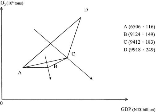
Fig. 1. Non-inferior solutions in the objective space.
find that the model has a good explanation ability and forecast performance. The empirical results show that the simulated domestic total output of 1994 is NT$ 13 621 billion, which is very close to the actual domestic total output, 13 633 billion
Žthe gap of estimation difference is only 0.05% . For the 1994 production level, the.
model shows that the simulated GDP for 1994 is also very close to the actual GDP
Ž .
in 1994 i.e. NT$ 6345 billion vs. NT$ 6376 billion . We therefore judge that the model accurate. Furthermore, the simulated GDP for 1996 is NT$ 7462 billion, while the actual GDP is NT$ 7492. Note that we estimate the CO emissions2
Žwithout restrictions in the year 2000 will be 249. =10 tons, representing 213% of6
1990 emission levels.
The objectives of the model as stated in the previous section are to maximize GDP and minimize CO emissions. We give each objective space for a dimension,2 which together form an objective space, as shown in Fig. 1. Beginning with the programming algorithm, we first maximize the single objective of GDP for the year
Ž .
at NT$ 9918 billion point D in Fig. 1 and the corresponding GDP annual growth rate is 6.85%. These results are similar to the Council for Economic Planning and
Ž .
Development’s CEPD 6.7% estimated growth rate for the year 2000 and an estimated GDP of NT$ 9670 billion. At this production level, the corresponding CO emissions are 2492 =106 tons, as mentioned above. This is the first non-inferior solution obtained.
In addition, we restrict CO emissions to 1990 levels and maximize GDP to2
Ž
derive the second objective which is a NT$ 6506 billion GDP for the year 2000
6 .
with a corresponding CO emission level of 1162 =10 tons for 1990 . This means
Ž .
Ž .
6506 billion 65.6% of NT$ 9918 billion for 2000 and that total domestic output will be NT$ 12 765 billion. Taiwan’s economy will be seriously weakened if the government seeks a policy of minimizing CO emissions. The annual growth rate2 would bey0.40%, which is lower than the government’s target of 6% plus. Here, we should indicate that zero GDP growth is not realistic, not to mention negative growth. Of course, the ideal solution is no CO emissions and a maximum level of2 GDP, which is naturally unattainable. Note that in this model, it is assumed that there is a constant percentage relationship between reduced CO emissions and its2
impact on GDP. If Taiwan reduces CO emissions by up to 120% and 140%, the2
GDP level in 2000 will decrease to NT$ 8933 and NT$ 9848 billion, respectively. This means 90.0% and 99.3%, respectively, of NT$ 9918 billion for 2000, where the respective economic growth rate would be 5.01% and 6.72%. This indicates that the greater the regulation of CO emissions, the stronger the impact on the2 economy. Also, Taiwan’s economy will show no deterioration if CO emission2
Ž 6 .
levels were up to 170% 197=10 tons .
We further derive the non-inferior solution by using the ‘center-point’ method,
Ž .
which was presented by Hsu and Tzeng 1992 . There are four non-inferior
Ž . Ž . Ž .
solutions Table 1 which match the derived points A 6516, 116 , B 9124, 149 , C
Ž9412, 183 , D 9918, 249 as shown in Fig. 1. These solutions represent the. Ž .
production levels of all the economic sectors in Taiwan and from the non-inferior solutions A, B, C, and D. We find that NT$ 2618 billion of GDP will trade off
6 Ž .
33=10 tons CO emissions between points A and B ; NT$ 288 billion of GDP2
6 Ž .
will trade off 34=10 tons CO emissions between points B and C ; NT$ 5062
6 Ž
billion of GDP will trade off 66=10 tons CO emission between points C and2
.
D . It is noted that solution A is a conservative policy, solution B and C are moderate policies and solution D is an aggressive policy. In solution A, Taiwan can attain the target of maintaining CO emissions at the 1990 level by year 2000, while2
Taiwan’s economy has an average y0.40% annual GDP growth. Taiwan’s govern-ment would not accept this solution. Conversely, in solution D, with NT$ 9918 billion GDP means a rapidly growing economy, showing an average of 6.85% GDP growth. If Taiwan chooses an economic policy like solution D, abundant CO2
Ž 6 .
emissions 249=10 tons would be produced and this solution would not be
acceptable to the IPCC. Solution C is similar to solution D, too. They can obtain 5.92% of annual GDP growth and means a relatively prosperous economy which has an impact on the economy of 5% or less. However, the corresponding CO2
6 Ž .
emissions are remain high, i.e. 183=10 tons 157% of the emissions in 1990 . This represents that if Taiwan’s government adopts this solution, rather difficult intra-country negotiations are needed. Finally, solution B is a good compromise option that Taiwan’s government could choose. The reason is Taiwan’s estimated
Ž
GDP in 2000, in this case, would only decline to NT$ 9124 billion 91.9% of NT$
. 6 Ž
9918 billion and have 149=10 tons of CO emissions in 2000 128% of the2
.
emissions in 1990 . Taiwan’s government can attain the above target by offering enough financial incentives to encourage investment activities related to CO2
mitigation and energy-saving matters.
()
T.
Chen
r
Energy
Economics
23
2001
141
᎐
151
147
Table 1
a
Ž .
Estimated results of four non-inferior solutions on Taiwan’s economy NT$ billion; %
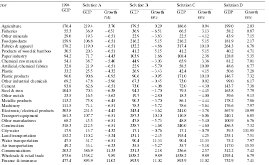
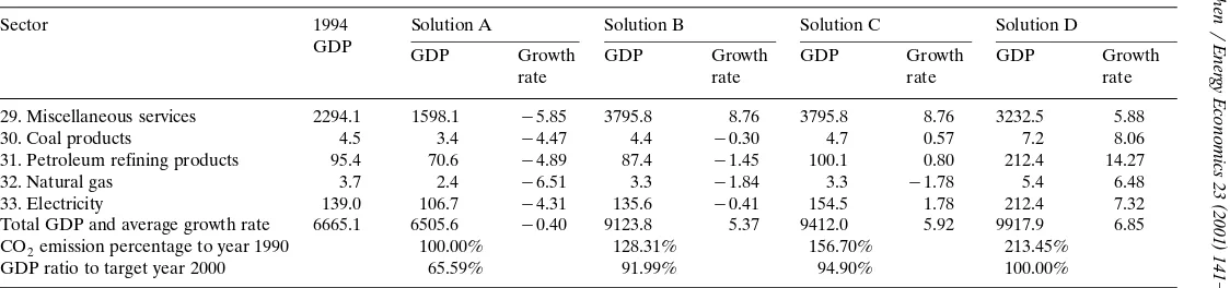
Sector 1994 Solution A Solution B Solution C Solution D
GDP GDP Growth GDP Growth GDP Growth GDP Growth
rate rate rate rate
1. Agriculture 176.4 219.4 3.70 179.5 0.29 186.6 0.94 199.0 2.03
2. Fisheries 55.3 36.9 y6.51 36.9 y6.51 66.5 3.13 58.2 0.87
3. Other minerals 29.0 19.3 y6.51 22.9 y3.83 22.5 y4.12 43.9 7.15
4. Food products 159.9 106.8 y6.51 216.2 5.15 216.2 5.15 181.9 2.17
5. Fabrics & apparel 178.2 119.0 y6.51 132.2 y4.86 317.4 10.10 264.3 6.78
6. Products of wood & bamboo 30.5 20.3 y6.51 41.2 5.15 41.2 5.15 40.2 4.71
7. Paper industry 94.2 71.7 y4.43 103.9 1.66 108.4 2.38 128.8 5.35
8. Chemical raw materials 54.1 38.7 y5.40 44.9 y3.03 65.9 3.36 81.2 7.01
9. Artificialrchemical fabrics 32.8 21.9 y6.51 22.9 y5.79 58.5 10.09 48.6 6.77
10. Plastic 33.2 25.5 y4.32 26.9 y3.43 42.4 4.15 50.6 7.28
11. Plastic products 96.0 90.6 y0.95 90.6 y0.95 171.0 10.10 146.7 7.32
12. Other industrial chemicals 69.2 47.8 y5.96 67.3 y0.45 73.0 0.92 99.0 6.17
13. Cement 93.8 62.6 y6.51 73.0 y4.08 72.0 y4.30 143.7 7.38
14. Steel & iron 104.5 70.3 y6.38 94.2 y1.70 79.5 y4.45 163.8 7.79
15. Other metals 23.5 16.5 y5.62 19.7 y2.80 18.3 y4.00 39.6 9.13
16. Metallic products 113.2 75.8 y6.45 90.3 y3.70 86.1 y4.44 178.2 7.86
17. Machinery 111.5 74.4 y6.51 78.3 y5.72 78.6 y5.64 176.6 7.97
18. Electronicrelectrical products 303.8 231.5 y4.42 243.4 y3.62 241.0 y3.78 567.9 10.99
19. Transport equipment 161.3 107.7 y6.51 287.3 10.10 110.8 y6.06 240.1 6.85
20. Other manufactures 68.2 45.5 y6.51 47.8 y5.73 48.8 y5.40 100.9 6.76
21. Construction 318.3 212.5 y6.51 238.7 y4.68 240.0 y4.60 486.3 7.32
22. City water 17.9 13.7 y4.32 17.1 y0.76 17.1 y0.79 39.3 131.95
23. Land transportation 152.2 110.2 y5.24 131.1 y2.45 195.4 4.25 235.1 7.51
24. Water transportation 47.5 31.7 y6.51 90.4 11.33 90.4 11.33 75.2 7.97
25. Air transportation 49.2 33.4 y6.23 35.5 y5.27 35.7 y5.18 117.0 15.55
26. Communications 203.2 386.9 11.33 231.3 2.18 236.6 2.57 312.2 7.42
27. Wholesale & retail trade 873.6 1538.2 9.89 1538.2 9.89 1538.2 9.89 1295.4 6.79
()
T.
Chen
r
Energy
Economics
23
2001
141
᎐
151
Ž .
Table 1 Continued
Sector 1994 Solution A Solution B Solution C Solution D
GDP GDP Growth GDP Growth GDP Growth GDP Growth
rate rate rate rate
29. Miscellaneous services 2294.1 1598.1 y5.85 3795.8 8.76 3795.8 8.76 3232.5 5.88
30. Coal products 4.5 3.4 y4.47 4.4 y0.30 4.7 0.57 7.2 8.06
31. Petroleum refining products 95.4 70.6 y4.89 87.4 y1.45 100.1 0.80 212.4 14.27
32. Natural gas 3.7 2.4 y6.51 3.3 y1.84 3.3 y1.78 5.4 6.48
33. Electricity 139.0 106.7 y4.31 135.6 y0.41 154.5 1.78 212.4 7.32
Total GDP and average growth rate 6665.1 6505.6 y0.40 9123.8 5.37 9412.0 5.92 9917.9 6.85
CO emission percentage to year 19902 100.00% 128.31% 156.70% 213.45%
GDP ratio to target year 2000 65.59% 91.99% 94.90% 100.00%
a
( )
T. ChenrEnergy Economics 23 2001 141᎐151 149
the impact of CO emissions will also be lessened. It is because Taiwan owns a2
Ž .
relatively high population 23 million among those countries, which have similar CO emissions. Empirical results indicate that Taiwan’s GDP in 2000 will decline2
Ž .
to NT$ 7708 billion 77.7% of solution D’s NT$ 9918 billion . The magnitude
Ž77.7% is slightly greater than the case mentioned above 65.6% . We further. Ž .
estimate that there will be 10.62 tonsrperson of CO emissions in 2000. It means2
Ž .
185% of the emissions in 1990 5.74 tonsrperson . Similarly, we can estimate a compromise solution like B. Taiwan’s estimated GDP in 2000, in this case, will only
Ž .
deduce to NT$ 9293 billion 93.7% of NT$ 9918 billion and there will be
6 Ž .
158=10 tons of CO emissions in 2000 124% of the emissions in 1990 . Taiwan’s2
government can choose it as an alternative option.
In this study, we find CO emissions have a significant mitigating impact in2 Taiwan. One of the reasons for this is that Taiwan has a high-income elasticity of energy. Taiwan’s average income elasticity of energy is projected to be 0.94
Ž1990᎐2006 , which is close to one and higher than that of countries of similar.
economic development like New Zealand and Israel. This shows that GDP growth in Taiwan over these years has almost been equivalent to energy use. Under the given magnitude of the coefficient of CO emissions, if Taiwan limits energy2 consumption in order to reduce CO emissions, its GDP growth rate will weaken2 proportionately. This also can be shown by the fact that energy-intensive industries are of huge importance in Taiwan’s industrial structure. However, Taiwan’s govern-ment and population have been attempting to promote energy conservation since the first oil crisis. Energy intensity so far in the 1990s is 11.38 LOErNT$103, which
Ž 3.
is better than that in the 1960s 13.19 LOErNT$10 and represents a continuous improvement. Achieving the goal of mitigating CO in Taiwan will require a strong2
effort in energy conservation both from the government and the people. It is suggested that the energy supply structure, manufacturing processes, and transportation system should be reformed towards less energy use and low CO2 emissions. In addition, for Taiwan to reduce CO emissions and energy imports, it2 needs to carry out economic restructuring by shifting its industrial structure from labor-and energy-intensive to less energy-intensive, high-technology, and light-en-gineering manufacturing industries such as household electrical appliances, electri-cal apparatus and bio-technologielectri-cal industries. Energy-intensive industries should not be encouraged and should only be developed in cases where there is good evidence that the products will be competitive at world prices. In the manufactur-ing sector, the steel, cement and chemical industries were the top three industries contributing to CO emissions. These industries also make up more than one-third2 of industrial GDP. There are three reasons for this. Firstly, the steel industry uses coal in its manufacturing processes; secondly, the cement industry uses lots of energy, being an energy-intensive industry; and thirdly, the chemical industry is also a high petroleum-intensity industry which utilizes a lot of energy. If Taiwan adopts CO emission regulations, it will significantly influence oil- and coal-related2
international cooperation for joint implementation of CO emission mitigation2 agreements, technology transfer to developing countries should be promoted. However, whichever policy or strategy is finally implemented will likely in reality implicate a trade-off between economic efficiency and environmental acceptability.
5. Concluding remarks
This paper employs a multi-objective programming model to evaluate the economic impact of mitigating CO emissions in Taiwan. We show that the costs2
incurred by CO emission controls are huge. Our empirical results show that,2
under CO emissions controls, Taiwan’s GDP will drop 34% off its maximized2 GDP objective for the year 2000 and that Taiwan’s economy will significantly weaken if Taiwan’s government stabilizes annual CO emissions at 1990 levels.2 Restrictions on CO emissions will reduce Taiwan’s annual average growth rate to2 2.44% in the period 1991᎐2000. This paper also shows Taiwan’s government has a choice of four non-inferior solutions to choose from in its efforts to tackle the CO2 emissions problem. In one of the solutions Taiwan’s estimated GDP for 2000 would
Ž .
only decrease to NT$ 912 billion 91.9% of NT$ 992 billion for the year 2000 with
6 Ž .
CO emissions of 149 10 tons 128% of 1990 emission levels . This solution would2 not significantly squeeze Taiwan’s economy and might be conditionally accepted by the international community. Taiwan’s government can also reach the CO emis-2 sions reduction target by offering financial incentives to encourage investment activities related to CO mitigation and energy-saving matters. One remark should2
be made here, the impact on Taiwan’s economy can be viewed as a kind of mitigating cost, which associated with CO emission reduction targets. Given the2 current state of technology, energy efficiency improvements and CO emission2 abatements, Taiwan will incur enormous costs from CO mitigation policy. If CO2 2 emission controls are indeed required, the incurred costs will have to be justified. However, there remain a number of uncertainties regarding the speed of techno-logical development and our understanding of future greenhouse effects. Taiwan, then, has a greater potential to reduce its actual expenditures. Therefore, it should be acknowledged that the empirical results derived in this paper are subject to several restrictions. For instance, the model is simplified in several aspects, some of them are planned to highlight the main points we are concerned with. In addition, the input data adopted in the model can never be perfect. The ‘penny switching problem’ also remains unsolved in programming models. That is, if the cost of
Ž .
technique R is slightly cheaper than the cost of technique S say, one penny , the solution of the programming model will totally substitute technique R for tech-nique S. This may not be the case in reality.
prefer-( )
T. ChenrEnergy Economics 23 2001 141᎐151 151
ences. In the process of economic and industrial planning, the managerial role of the government should be taken into account. The economy could perform better if government were appropriately involved. However, one point should be kept in mind, i.e. solutions and conclusions of this type of model imply an ‘optimum’ which is generally ‘better’ than the real situation. In practice, the economy may always perform less than the optimum due to poor management or unmanageable factors. The conclusions arising from these empirical findings imply the direction of government efforts towards a better situation.
However, in order to limit CO emissions, Taiwan’s government should adopt2
some appropriate strategies. The top strategic priorities could be the efficient use of energy, introduction of non-fossil fuels, international cooperation on joint implementation, and the introduction of innovative technologies. It is worth conducting a further study to establish several policy alternatives to simulate the above findings in the near future.
References
Fells, L., Woolhouse, L., 1994. A response to the UK National Program for CO emissions. Energy2 Ž .
Policy 22 8 , 666᎐684.
Hafkamp, W.A., Nijkamp, P., 1982. An integrated interregional model for pollution control. In:
Ž .
Lakshmanan, T.R., Nijkamp, P. Eds. , Economic Environmental Interactions Modeling and Policy Analysis. Martinus Nijhoff, Boston.
Hsu, G.J.Y., Tzeng, L.Y.R., 1992. A new algorithm of multi-objective programming: the center-point
Ž . Ž .
method. J. Manage. Sci. 9 1 , 39᎐50 in Chinese .
Ž .
Loucks, D.P., 1975. Planning for multiple goals. In: Blitzer, C.R., Clark, P., Taylor, L. Eds. , Economy-Wide Models and Development Planning. Oxford University Press, London.
Manne, A.S., Richels, R.G., 1991. Global CO emissions reduction: the impact of rising energy costs.2 Ž .
Energy J. 12 1 , 87᎐107.
Ž .
Morrison, M.B., Brink, P., 1993. The cost of reducing CO emissions. Energy Policy 21 3 , 2842 ᎐295. Ž .
Nordhous, W.D., 1992. The cost of slowing climate change: a survey. Energy J 12 1 , 37᎐65.
Nijkamp, P., 1986. Equity and efficiency in environmental policy analysis: separability versus
inseparabil-Ž .
ity. In: Schnaiberg, A., Watts, N., Zimmermann, K. Eds. , Distribution Conflicts in Environmental-Resource Policy. Gower, London.
Rose, A., 1995. Global Warming Policy, Energy, and the Chinese Economy. Pennsylvania University Press, Pennsylvania.
Rose, A., Steven, B., 1993. The efficiency and equity of marketable permits for CO2 emissions. Resource Energy Econ. 15, 117᎐146.