METHODS
ECECMOD: an interdisciplinary modelling system for
analyzing nutrient and soil losses from agriculture
Arild Vatn
a,*, Lars Bakken
b, Peter Botterweg
c, Eirik Romstad
a aDepartment of Economics & Social Sciences,Agricultural Uni6ersity of Norway,PO Box5033,1432Aas,NorwaybDepartment of Soil & Water Sciences,Agricultural Uni6ersity of Norway,PO Box5028,1432Aas,Norway cCenter for Soil & En6ironmental Research,1432Aas,Norway
Received 2 December 1997; received in revised form 9 September 1998; accepted 22 October 1998
Abstract
This article discusses a set of principles for policy analysis of environmental problems. The main focus is on integrating economic and ecological analyses through a mathematical modelling framework. The paper starts by developing a general model for the study of environmental issues. Principles for operationalizing the model are discussed, and ECECMOD (a new modelling system constructed to analyze pollution from agricultural systems on the basis of these principles) is introduced. Some of the results obtained by ECECMOD are presented to facilitate a discussion about the gains to be obtained by this kind of analysis. The study shows that it is of great importance to combine economic and ecological analyses at a fairly high level of resolution when studying environmental effects of complex systems. © 1999 Elsevier Science B.V. All rights reserved.
Keywords:Eco-eco modelling; Interdisciplinary research; Environmental regulations; Nitrogen; Erosion.
www.elsevier.com/locate/ecolecon
1. Introduction
Environmental problems are characterized by interactions among societal institutions, resource use choices made by economic agents within these institutions, and the different natural processes these choices influence and are influenced by. In this light it is disturbing that most studies (even
those addressing environmental policy issues) have been undertaken within single disciplines. Given the character of the problem, such a strat-egy runs the risk of producing research with low cross-disciplinary coherence and little policy rele-vance (Vatn et al., 1997).
The background of the study presented here is the North Sea Treaty mandating that the coun-tries of the area reduce nutrient emissions to the sea by 50%. Given the problem, we were ‘forced’ to find practical and productive ways of integrat-* Corresponding author.
ing relevant sciences. It turned out to be a chal-lenge both to integrate and to maintain the qual-ity standards of the involved disciplines. We experienced (in a very concrete way) why interdis-ciplinary research is so rare.
To be able to communicate coherently across the fields of study, we had to find a common language and scientific structure. We found that mathematical modelling could facilitate that. Our first step was to develop a general model for studying policy choices concerning pollution and degradation of natural resources such as water, air and soils. Next, we had to find ways of making the model operative and of developing an analysis tool by which empirical studies in the field of nutrient losses from agriculture could be under-taken.
In this paper we present the most important steps of the process of model construction, illumi-nating the various conflicts that arise when inte-grating across disciplines. Further, we introduce the interdisciplinary modelling system that was finally developed (ECECMOD) and present some of the results obtained using this system. Since our focus is methodological, we will concentrate on results illustrating the potential of integration and the gains that can be obtained by using rather detailed analysis with high levels of resolution. For those interested in a more comprehensive overview of the results, we refer to Vatn et al. (1996, 1997).
2. A general and idealized model
From an economics point of view, pollution problems are considered to be incentive problems. Economic agents do not face all costs associated with their activities. For natural scientists, pollu-tion is primarily about changes in matter cycles, cumulative or disruptive changes in various eco-systems where the ‘actors’ are ions, bacteria, fish, etc., operating at very different scales compared to the economic ‘actors’. In order for the potential consequences of certain policies to be foreseen, the different levels/subsystems involved need to be well linked and the right levels of resolution cho-sen. The problem, as we see it, is that economists
in their analysis primarily utilize very simplified assumptions about the natural world, and the natural scientists hardly take into account the fact that in formulating policies one has to consider motives, constraints, and institutions determining human choices.
From an economic perspective, a pollution problem is of interest if there exists a potential for welfare improvement by institutional changes re-sulting in less pollution. Coached in a principal-agent framework and assuming the principal-agents to be expected profit maximizers, the policy problem may be formulated in the following general way: Principal:
To simplify the exposition, all agents (i) are considered to be firms, and each firm owns a homogenous element (i) of the natural assets z. The arguments in the social welfare function W
consist only of the present value of agents’ in-comes (profitsp) and the states of the recipient r. The emissions are here considered to be global (e.g. the location of the emission does not influ-ence its effect). Following the standard Pigovian policy solution, the principal’s choice variable is a set of firm-specific taxes on emissions equal to their marginal environmental costs. The tax changes the incentive structure the agents are facing, as the costs they impose on others become part of their optimization calculus.
Eq. (1c) contains little information about the structure of the agent’s decision problem and the dynamics of the environment. A more complete formulation is given in Eqs. (2a), (2b), (2c) and (2d):
and where: x denotes a vector of variable inputs used; b denotes a vector of fixed inputs in the form of man-made capital;qdenotes a parameter for the quality of the chosen technology; g de-notes a function for the productivity of the natu-ral assets z; u* denotes a vector of optimal environmental taxes obtained through solving Eqs. (1a), (1b) and (1c);k denotes a function for the terminal value of assets b and z; l denotes a function for the effects of agents’ choices and
previous states of z and r on the state of the natural assets r; m denotes a function for the effects of agents’ choices and previous state of z on emissions; and s denotes a function for the relation between emissions and the state of the recipient.
Eq. (2a) is formulated as a standard profit maximization problem for agent (i) given that it faces a set of environmental taxes (u*) and has access to natural resources zi. The input vectorsx and band technology (q) are specifications of the vector ø of choice variables as depicted in Eq. (1c).
The dynamics of the natural system which the agent influences through choices about inputs (x, b) and technology use (q), are described by Eqs. (2b), (2c) and (2d). As to assets, a distinction is made between man-made capital b and natural assets zandr. Elements ofzare used as inputs in production, while r describes the state of the recipient. The distinctions are purely analytical, and what is a recipient (r) for one agent may be the resource (z) for another. Thus, the dynamics of emissions, the state of the recipients, and the quality of the resources are influencing each other in complex and time dependent ways. This is taken care of by Eq. (2c) where the elements of z at time t depend upon previous capital invest-ments (inbandz) and the changes in the recipient r (Eq. (2d)).
Through the specification of zandt, the model incorporates variation both in space and time. In the case of biologically based production systems, the productivity of the resources may vary sub-stantially due to variations in the quality of soil and water and the variability in weather. The weather will only be known with certainty ex post. The agent must therefore make decisions on ex-pected profits, justifying the use of the expectation operator E in Eq. (2a).
3. Principles for operationalizing the general model
and (2a) to (2d)). In general there are important trade-offs to be made between preserving some complexities while reducing others.
First of all, agents are not necessarily profit maximizers, even though most production analy-ses assume this. They may both have a more complex preference structure (utility maximiza-tion, risk aversion ( Nakajima, 1986; Singh et al., 1986)), and they may not (always) maximize. They may use satisficing rules or follow specific behavioral norms developed among practitioners in the field (Simon, 1979; Hodgson, 1988; Vedeld, 1998). Profit maximization still has high merit, as it is chosen also because it is easier to handle analytically, avoiding further complications in an already very complex model structure.
Environmental taxes in Eqs. (1a) to (1c), and (2a) to (2d), assumed to be assigned to emissions, as in the standard point-source pollution case. This is not an obvious solution, since emissions often are non-point and variable. In most cases where renewable natural resource use is involved, the non-point character of emissions renders the costs of gathering necessary information to under-take emission based regulations prohibitively high. This introduces an extra complication for the principal, since measures may either have to be assigned to input factors (x or b), or to the way these factors are combined internally and with z through defined technologies (q). In our case we found it necessary to address these complications.
The complexity of the problem will often make it difficult to determine optimal levels of the pol-icy control variables in u. It is sufficient to men-tion the problems of valuing environmental functions (Hausman, 1993; Vatn and Bromley, 1994). Thus a full cost-benefit analysis may be very difficult and, even obscure the problem. An alternative then is to use a cost-effectiveness crite-rion, measuring costs for obtaining certain levels of emission reductions. Technically speaking this implies omitting the optimization problem defined in Eqs. (1a) to (1c) and instead produce informa-tion for the principal through a scenario type modelling. Here the effect of various levels of the policy vector u on p, z, d and r is explored utilizing the equations in Eqs. (2a) to (2d) only.
We chose to use this type of sequential search procedure. This does not necessarily reduce infor-mation quality. Rather, it may make the results more transparent, as it also makes it easier to preserve higher resolution especially in the natural science part.
Given the above simplifications, one is still faced with the problem of describing and linking processes (and thus disciplines) demanding analy-ses at widely different scales. Moreover, one has to find tractable ways of solving an optimization problem with the complicated dynamics and feed-backs described in Eqs. (2a) to (2d). Let us ad-dress these issues.
3.1. Integration across scales
While economists do their analyses at the level of the firm, a sector or the society, natural scien-tists normally undertake their analyses within geo-graphically localized, often rather small-scale-specified, physical and/or biological conditions. These differences are caused both by variations in scope and by the type of processes studied (Antle and Capalbo, 1993).
A way to overcome the problem of varying scales and foci is to utilize the fact that natural systems tend to be organized in hierarchies (O’Neill et al., 1986). Processes are nested, with those at one level becoming elements of those at higher. The problem becomes one of maintaining the necessary non-linear fine-scale variation as one moves upwards into more coarse-scale aggre-gations. Rastetter et al. (1992) discuss three meth-ods by which to accomplish this:
a. partial transformation using an expectation operator to incorporate fine-scale variability; b. partitioning — separating the coarse-scale
ob-jects (aggregates) into a manageable set of relatively homogeneous subgroups; and c. calibration — recalibrating fine-scale data to
coarse-scale information.
useful-ness of method (c) rests on the availability of data both at the fine and coarser scales, and is difficult to use if the aim is to study effects of changes in a system.
As Costanza et al. (1995), we find partitioning to be a good solution for analyses of land-based systems. Here the various resources or decision units are classified into homogenous groups at relevant levels and integrated in a hierarchical structure. This way partitioning offers a sur-veyable platform for linking analyses that must be undertaken at different levels and studied with various resolutions.
Linking across levels means to a large degree linking across disciplines. While natural hier-archies exist, it may still be difficult to identify aggregates that serve both the ‘aggregate’ and the ‘disaggregate’ sciences well. Partly, this reflects disciplinary traditions, but it may also reveal real discontinuities. These kinds of problems are espe-cially prone to occur as one crosses over from the natural to the social sciences. We will return to this issue later.
3.2. Sol6ing the optimization problem
The optimization problem in Eqs. (2a) to (2d) is formulated as an optimal control problem in dis-crete time. The complexities, especially in the underlying structure of the natural processes, will however often prohibit solving Eqs. (2a) to (2d) simultaneously. Reducing complexity may not be justifiable. Two partial solution concepts that stand out are:
1. Iteratively solving each equation in Eqs. (2a) to (2d) for relevant sequences of time, updat-ing the equations with necessary information from each other.
2. Modelling for the whole time period in two sequences — first agents’ choices, then the ef-fect of these choices on the natural processes. To cover important feed-backs, the natural science information necessary to solve agents’ optimization problems are produced initially under simplified assumptions about agents’ choices/practices.
The merits of these two methods depend on the problem, the type of dynamics and the role of
time. Method 1 takes best care of the interactions between the different levels of the system — the dynamics between the economic and ecological parts. For large systems, iteration will tend to be very resource demanding, and it will by definition not be possible to solve the economic optimiza-tion problems simultaneously for the defined pe-riod of analysis.
According to procedure 2, the agents’ optimiza-tion problem will be solved given rather coarse pre-estimated information about developments in the natural processes. Thereafter, the equations describing the natural asset dynamics are solved at the most desirable level of resolution and on the basis of information about the model agents’ choices of production practices. Agents’ informa-tion about the development of the natural re-sources are often coarse and uncertain at the time of decision. Procedure 2 actually mimics that fea-ture, as it also is the easiest to implement if high resolution in the natural science part is necessary. We have chosen method 2 in our analysis.
4. ECECMOD — The economics and ecology modelling system
To demonstrate how the above principles may be utilized, we will turn to a presentation of ECECMOD — a modelling system established to study the effect of different policy measures on mineral emissions from agriculture. The system is fully documented in Vatn et al. (1996) and con-sists of a set of process-based, interlinked models. Some are constructed specifically for the project, while it has been possible, in other cases, to build on existing models.
4.1. The agronomic system and nutrient losses
Nitrogen and phosphorus are essential elements of mineral fertilizers added to enhance plant pro-duction in agriculture. If lost to the environment, the same elements represent a potential pollution problem. They may cause eutrophication in fresh and/or coastal waters. Nitrates may reduce groundwater quality, induce acidification and, in the form of N2O, affect the ozone layer and
global warming.
Phosphorus displays more local effects, while nitrogen in different compounds influences the environment both at the local level and on a global scale. Nitrogen is a dynamic and elusive element in nature. Therefore, both the form and magnitude of losses depend on a series of condi-tions such as weather, fertilizer levels, plant up-take, incorporation of organic matter into soils, utilization of manure N, etc. Supplies of mineral N during the growing season is a prerequisite for successful plant production. Nitrate (NO3−) is a
very mobile ion, making it a preferred N-source in plant production, but also prone to leaching. Losses may be decreased by reducing the input of mineral N. However, both plant uptake and soil processes affect losses greatly. This implies that to control losses, one must look at the agronomic practice as a whole.
Plant roots are by far the strongest mineral N sink in the soil. The response of plants to N fertilization is crucial in predicting the relation-ship between fertilizer levels and nitrate leaching (Vold et al., 1994). Crop failure due to drought periods in rainfed agriculture results in large N losses through leached residual nitrate out off season (Uhlen, 1989).
The soil and the heterotrophic soil microflora (+fauna) are other potential sinks. N incorpo-rated in organic soil compounds represents a large pool of nitrogen in the system — 20 – 100 times the annual doses of mineral fertilizers. Depending upon the supply of energy through plant residues and/or the type of tillage system used, the mi-croflora functions either as a net sink or net source of mineral N. Due to the stability of the organic components involved, a net increase or decline in the soil organic N pool may continue
for decades, depending on the agronomic practice (Christensen and Johnston, 1997).
The annual changes in soil organic N may be moderate compared to the total amount in the soil, but large in relation to the nitrogen inputs (fertilizers) and outputs (crops) from the system. Soil texture has a profound influence on the level and changes in soil organic nitrogen (ibid). This role of soil organic N invalidates N budgets as a criterion for the environmental performance of an agronomic system with normal N inputs. At the same time it constitutes an important rationale for choosing a process-oriented N modelling ap-proach with a high resolution both in time and space when analyzing the effects of policy mea-sures for reducing nitrate leaching.
Phosphorus is much less elusive than N, as it is strongly bounded to soil mineral fractions. Since losses are to a large degree the result of erosion, the input of mineral phosphorus through fertiliz-ers has little impact on losses, at least for short and intermediate time spans. Plant cover, tillage practices, etc. are far more important for erosion and resulting P-losses than input/output relations. Thus even this case shows how important it is to understand the dynamics of the agronomic prac-tice as a whole. Further, the impacts vary sub-stantially with differences in soil characteristics and topographical conditions. In the case of soil erosion, losses are highly episodic, due to the importance of precipitation.
4.2. System,le6els and processes
considered homogeneous within each catchment, in practice often implying necessary division into subcatchments. While few economic units are defined by watershed borders, they are capable of subsuming a number of production units fairly well.
Using partitioning as the basic method for pre-serving the necessary variation and for nesting levels, we observe that farms, soil types, and topography are important spatial elements of variation. Farm size, type of production, and stocking rates are notable sources of diversity at the farm level. Nitrogen turnover, plant growth and P losses vary with climate, soil types and topography, the latter influencing water erosion. Based on this, we chose the following levels and partitioning criteria:
1. Watersheds/catchments. Partitioning criteria: Weather conditions, topography and produc-tion. Modelling: Aggregated emissions to air and water.
2. Farm. Partitioning criteria: Farm size, type of production, and stocking rate. Modelling: Farmers’ choices of agronomic practices. 3. Farm field. Partitioning criteria: Soil
proper-ties and chosen agronomic practice. Mod-elling: Crop growth and farmers’ choices of agronomic practice; hydrology, nutrient (N) turnover and leaching.
4. Plot/grid cell. Partitioning criteria: Topogra-phy, soil properties, slopes, and agronomic practice. Modelling: Erosion and P-losses. With regard to the time dimension, it was nec-essary to combine high resolution (episodic na-ture) with long simulation periods (variation). The total length of the analysis period is set at 20 years. Farmers’ decisions are dominantly mod-elled at the level of years or seasons (choice of crops, tillage practice etc.), but in some cases at the level of days (sowing dates, etc.). Each of these decisions is modelled consistently with the information resolution of the corresponding deci-sion problem. The natural science modelling is mainly undertaken at the level of days. In the erosion analysis, the basis is rainfall events that may have durations from minutes up till several hours.
4.3. The structure of the modelling system
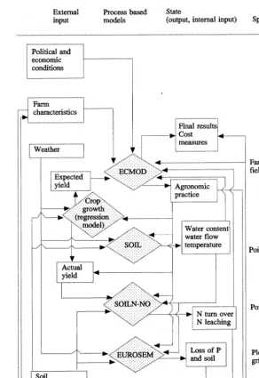
ECECMOD consists of a set of linked submod-els covering the different parts of the system as described in the above hierarchy. As the mod-elling system now works, the optimization prob-lem in Eq. (2a) is solved on a year by year basis. This is due to capacity constraints. It does, how-ever, represent a minor problem in our case, since the terminal value of the relevant assets (e.g. soil and soil N volume) is not considered to influence the choices studied.1 Fig. 1 gives an overview of
the main structure of ECECMOD.
The figure differentiates between external in-puts, (process based) models, and model outputs (intermediate and final states). The level of resolu-tion (scales) for the space and time dimensions is also given. The analyses are driven by a set of input data defined by farm structures and soil and weather conditions in the actual catchment. By changing the institutional setting within which farmers’ decisions are to be made, it is possible to analyze the effects on emissions and the costs implied. Thus far the effects of the emissions on down-stream water-courses is not integrated into the model.
As to the different parts of the system, we would emphasize the following:
ECMOD is an optimizing model operating at the farm level. The optimizing problem to be solved follows in principle the formulation in Eq. (2a) with constraints related to acreage and labor. The policy variable is (as already emphasized) formulated differently though, as taxes or other types of regulations are attached to inputs (x or b) like fertilizers, or to the management practices (q) like plowing time, catch crop use2, storing
facilities for manure, etc. and not to emissions. ECMOD consists of a set of modules solving the choice problems that are assumed to be the
1For example, farmers are, under Norwegian conditions, not considered undertaking soil mining — a point where the model formulation actually deviates from a strict net profit maximizing rule.
Fig. 1. The structure of ECECMOD.
ones influencing emissions the most. These are the setup of machinery, choice of crops and crop rotation, fertilizing levels, manure practices (both storing and spreading), soil tillage, and sowing dates. The optimizing procedures are mainly non-linear and based on expectations where relevant. The model also calculates economic parameters to be used when estimating the cost-efficiency of different strategies.
SOILN – NOis also a one-dimensional, layered deterministic model describing nitrogen turnover (Johnsson et al., 1987; Vold, 1997). It produces information about loss of N as a function of agronomic practice, plant growth, weather, and soil characteristics (soil type and agronomic his-tory) expanded from point to field level assuming homogenous fields. The modelling of the micro-bial N-transformations has been found to respond adequately to various physical and chemical fac-tors, and to various litter types (Vold et al., 1994; Vold, 1997). Parameterization of the plant N up-take function is based on regional agronomic experiments (yield and N uptake) and regional annual yield statistics. It is estimated as a set of non-linear functions with yield and available N as arguments with good fit (R2 for single crops
varied from 0.82 to 0.92; Vold et al., 1999). Pre-runs are undertaken to estimate the effect on N-mineralization of changed manure practices, catch crop use, etc. for use in ECMOD.
EUROSEM describes erosion as a function of agronomic practice, weather, soil characteristics and local topography. It is an episode-oriented, process-based model substantially diverging from the more dominant tradition of regression-based analyses (Botterweg, 1998; Morgan et al., 1998). It is used to produce estimates for soil losses as a function of soil characteristics, topography, agro-nomic practice, and weather conditions.
Landscape models. Finally, two systems or models for aggregating data from plot and/or field level to the level of watersheds are developed. The aggregation of costs and N leaching estimates is a fairly simple weighing based on the relative distribution of productions, soils, etc. in land-scapes. For erosion, GRIDSEM (Leek, 1993) is used to estimate mass transport in landscapes, aggregating losses over whole watersheds as a function of estimated losses at each plot/grid cell (from EUROSEM), the distance from plot to surface waters, and topographic characteristics over this distance (Botterweg et al., 1988).
ECMOD is run for a set of representative model farms covering the variation in each catch-ment. The actual farms in the area are partitioned into groups defined by what is considered the most important variables in our case — e.g. type
of production, farm size and amount of manure (total and per ha). For each of these groups a model farm is defined, generally based on the mean values for various parameters for the under-lying real farms. Each model farm is divided into fields with representative soil characteristics. The landscape is divided into series of plots/grid cells homogeneous in soil type and slope. To be able to transfer information about agronomic practices from the analyses at the model farm level back to the landscape level, each plot is attached to a model farm field on the basis of soil properties and which partition of real farms it belongs to. The methodology chosen thus demands data about the location of each farm and extensive landscape information.
4.4. Partitioning and interaction — crop growth as an example
The way crop growth is modelled illustrates the manner in which different levels of ECECMOD interact. The functionfin Eq. (2a) is developed in the following way:
Y=fijkt(N1t,N2t,N3t)*VatP (3)
where: Y denotes yield as dry matter; i denotes model farm field/type of soil; j denotes type of crop;kdenotes climate zone;tdenotes time (year or season); N1t denotes nitrogen in mineral fertil-izers applied at time t;N2t denotes nitrogen from manure in mineral form (ammonia) applied at time t; N3t denotes mineralized N from the or-ganic components of the soil at timet;Vatdenotes
an operator covering the effects of different ele-ments of agronomic practice except fertilizing; and P denotes phosphorus in fertilizers.
The production function is partitioned by soil, crop, climate zone and year, the latter to capture weather dependent variation between years. Fur-ther, it is structured so that mineral N is the only argument in the production function, while the influence of other elements onf(·), is taken care of by the operatorVat. The N component is divided
produc-tion funcproduc-tion of Eq. (2a) are either kept con-stant (e.g. incorporated into f) or they are taken into account by Vat.
The function fijkt is estimated on the basis of trial data for an agronomic practice using fall tillage and mineral fertilizers only. Changes in tillage practice, sowing date, use of cover crops, etc. are taken into account by Vat inducing
changes in the parameters of fijktrelative to their estimated effects in trials. This illustrates that the structure is chosen also to facilitate the use of data from factorial trials in a more dynamic type of modelling.3 As Eq. (3) is structured,
changes in mineralization (N3) due to the use of
animal manure, catch crops etc. is captured in a way that also influences the optimal use of fer-tilizers in the form of N1 or N2. The level of N3
is established on a more coarse scale than in the final N modelling — e.g. the average values for the whole 20-year period is used. The data is produced through pre-estimations by running SOILN – NO under different standardized catch crop regimes.
The crop growth module illustrates a major difference in needs between economics and the natural sciences. While the plant growing pro-cesses must be modelled following the actual weather, the farmer makes decisions mainly on expectations about the weather and subsequent crop growth. This distinction is taken care of by estimating annual production functions to be used in the natural science part of the modelling (fijkt) and an average function used to represent the expectations of the farmer (fijk). This demonstrates that modelling economic choices at a coarser scale than the N dynamics may often be the appropriate choice, representing no infor-mation loss compared to the real world situa-tion. In some cases (as in the study of a split fertilizing regime) we allow the farmer to update
fijk with information about weather development between the different applications to secure con-sistency.
5. The gains of high resolution eco-eco modelling
To illustrate some of the gains of the type of analysis advocated here, we will turn to a selected group of results from a study undertaken for two catchments in southeastern Norway. A series of research objectives has been formulated focusing on the cost-effectiveness of input regulations ver-sus regulating the agronomic practices. Since nat-ural conditions and types of production vary substantially among farms and regions, it is of special interest to analyze gains and losses related to uniform versus differentiated policy measures.
5.1. The study sites
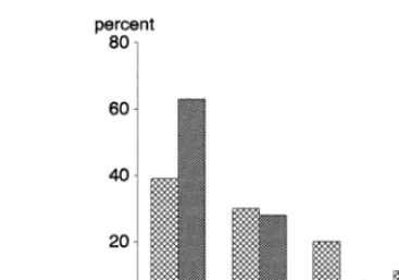
The analysis covers the Mørdre catchment and a subsection of the Auli catchment in the counties of Akershus and Vestfold, respectively. The amount of arable land in the Mørdre catchment is approximately 450 ha and in Auli 2.600 ha. Both areas are dominated by grain production, while there is some animal production especially in the Auli area. The distribution of soil types is very different in the two catchments (Figs. 2 and 3).
While clayey and sandy soils dominate in Auli, silty soils dominate in Mørdre. Auli has a higher mean annual temperature (6.3°C compared to 4.2°C) and precipitation (1009 mm compared to 809 mm). In both areas, grain is the most impor-tant crop. However, Auli has a much larger pro-portion of animal husbandry. The amount of manure N per ha is on average ca. 75 kg in Auli and 18 kg in Mørdre.
5.2. Strategies for reducing nitrogen emissions.
Various types of regulations directed either to-wards inputs (x,b) or the farming practice (q) are available to the authorities. Analyzing this we distinguish between ‘physical’ measures which are the changes farmers undertake in the way they farm, and ‘policy’ measures which are the instru-ments the authorities use to motivate or compel farmers to change practices. According to the dynamics of the plant-soil system (z) in grain producing areas like ours, we grouped physical measures into four categories:
reduced total nutrient input (lower ‘intensity’, better manure practices, etc.);
improved adjustment of nutrient input (espe-cially of N) to yearly growth condition (split fertilizing, etc.);
changed tillage practices and/or continuous plant cover (catch crops) etc. to reduce erosion and enlarge the plant N uptake period; and increased rates of N immobilization in the soil
in periods where crops are not grown (incorpo-ration of catch crops, straw, etc.).
Policy measures to accomplish the above changes may be a tax on mineral N fertilizers (fertilizer intensity/manure handling), seasonal quota system (split fertilizing), mandatory or sub-sidized practices (changed tillage practices and catch crops). The interactions covered by ECEC-MOD make it possible to account for a wide range of both direct and indirect effects in the system, related to changes in agronomic practices and losses of nutrients. Many of these effects could hardly have been studied through a more aggregate procedure, and in some instances the effect of preserving high resolution turns out to be profound. Through the following presentation of results, we will try to illuminate the role of pro-duction type, choice of crops, choice of technol-ogy, soil characteristics, soil dynamics and topography.
5.3. Comparing different policy measures
To compare policies, a set of scenarios was constructed. To validate the modelling system, a
Fig. 3. Distribution of production types in Auli and Mørdre, farms classified by dominant production.
scenario covering the actual policy conditions in 1992 was run. Compared with available data, the results were very encouraging both concerning chosen agronomic practices and leaching levels. The fit for yearly and average yields, fertilizer levels and choice of crops was very good, with deviations of only a few percent. The level of spring tillage was somewhat over-estimated, whereas the opposite was the case regarding ma-nure storing capacities (for more specific docu-mentation see Vatn et al., 1996). As to leaching and erosion, we encountered some problems with acquiring spatially comparable observational data. Data both from smaller parts of the catch-ments and lysimeter expericatch-ments have been uti-lized. Except for the lysimeter trials, direct comparisons are difficult to do. For these trials model fit was in general found to be very good, except for abnormally high fertilizer level treat-ments (Vold, 1997). Concerning erosion and P losses comparisons with field observations was utilized, showing deviations normally within a range less than 920 – 30%.4 Estimated level of P
losses in Auli were the ones deviating the most. For more specific documentation see Botterweg (1998) and Vatn et al. (1996).
Next, a Base scenario was run. Again the refer-ence was the policy conditions in 1992, but exist-ing environmental regulations were ignored to formulate the best basis for comparing various
Fig. 2. Distribution of soil types in Auli and Mørdre.
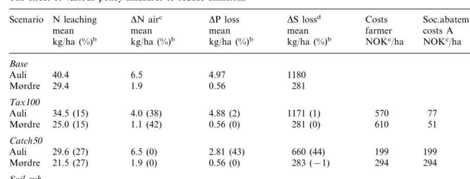
Table 1
The effect of various policy measures to reduce emissionsa
DS lossd
Scenario N leaching DN airc Soc.abatem. Soc.abatem.
DP loss Costs
mean mean mean mean farmer costs A costs B
NOKe/ha
kg/ha (%)b kg/ha (%)b NOKe/ha NOKe/kg Nf kg/ha (%)b kg/ha (%)b
Base
6.5 4.97 1180
Auli 40.4
1.9 0.56 281
29.4 Mørdre Tax100
4.0 (38) 4.88 (2) 1171 (1)
Auli 34.5 (15) 570 77 13
1.1 (42) 0.56 (0) 281 (0) 610
25.0 (15) 51
Mørdre 12
Catch50
6.5 (0) 2.81 (43) 660 (44)
Auli 29.6 (27) 199 199 18
1.9 (0) 0.56 (0) 283 (−1) 294
21.5 (27) 294
Mørdre 37
Soil-sub
6.5 (0) 2.25 (55) 505 (57) −370 138
Auli 40.0 (1) 370
1.9 (0) 0.55 (2) 2.77 (1) −510 30
29.5 (0) g
Mørdre
aEstimated costs and changes in emissions as compared with the Base scenario. bPercent reduction from Base.
cLoss of ammonia-N in connection with manure spreading. dSoil loss.
eNOK=Norwegian kroner. fCosts per Kg reduced N leaching. gIrrelevant since N leaching is increasing
policy options. We will start by comparing the results from the following scenarios:
Tax100: 100% tax on N-fertilizers;
Catch50: 50% arable land requirement on catch crops or grass cover; and
Soil-sub: A per hectare subsidy for spring/no tillage (1992 level: 1000 NOK per hectare). While the tax has to be uniform for the entire economic – political area (in our case the whole of Norway) the other measures can be differentiated between regions if desirable.
The results (including the Base scenario) are given in Table 1. The estimates are produced on the basis of weather data for each area for the period 1973 – 1992. The table shows a fairly broad array of environmental indicators, making it pos-sible to analyze trade-offs involved. Estimates are given for N leaching, NH3 losses to air, P losses
and losses of soil. A set of cost-efficiency mea-sures is also presented. ‘Farmers’ costs’ shows average reductions in profits per ha as measured against the Base scenario. Two average social cost-efficiency measures (defined as ‘Farmers’ costs’ exclusive environmental taxes/subsidies) are
presented. Since there are several types of emis-sions with no obvious common yardstick, a per ha measure is given (‘social abatement costs A’). In the case of ‘social abatement costs B’, all costs are carried by the N-leaching — the dominant form of N emission. Costs related to policy administration are not included. This will be addressed later.
Starting with the Base scenario, we see that the estimated agronomic practices and losses differ between the areas. The higher level of leaching in Auli is mainly due to the level of animal manure and the rather large proportion of sandy soils, which are most prone to leaching. The low soil loss in Mørdre is explained by differences in slope characteristics, as well as the dominance of silty soils. These soils are generally tilled in spring since that produces the highest yields. Spring tillage reduces erosion.
of Soil-sub in Mørdre is mainly explained by the mechanisms keeping losses in the Base sce-nario down.
Catch50 reduces both N-leaching, P and soil loss. It could thus seem to be a good alternative in areas where all the measured types of losses are of importance. The effect of Catch50 on N-leaching is quite substantial, illustrating that losses can be reduced considerably if one is able to continue plant uptake for a longer period of the year. Reductions in inputs are thus not the only interesting options for reducing N losses. For the most part, nitrogen taken up by catch crops enters a pool of stable organic compounds after ploughing. This pool has a decay rate (first order decay) of about 0.01 per year (Vatn et al., 1996, pp. 55 – 67). This implies that the system is able to accumulate N in this pool for several decades before returns (as humus-derived min-eral N) becomes a significant contributor to the mineral N supply. A separate model study showed that the catch cropping will reduce the mineral N supply to the cash crop for a period of some 30 – 40 years. This actually results in increased optimal N fertilizer (N1+N2) levels.
After this period the soil starts ‘paying back’ and the level of fertilizers can then be reduced (Vold et al., 1995).
Looking at the costs, the tax entails the low-est social abatement costs if we only consider N-leaching. The reductions in P and soil losses following the two other measures, may still be considered large enough to outweigh the higher per hectare costs, especially in the case of catch crops. We observe that farmers’ costs and social costs are identical in the case of Catch50, while in the tax scenario, the tax counts for about 90% of farmers’ costs. The observed income gain (negative costs) for the farmer in the case of Soil-sub, indicates that the subsidy was set higher than necessary to motivate farmers to re-duce fall tillage. The table illustrates that the distributional effects can be substantial depend-ing on the type of policy measures used (taxes, requirements or subsidies).
Catch crops are less effective in Mørdre than in Auli. The social abatement costs are 50 – 100% higher than those of the latter. Several
factors cause this. The lower initial level of leaching plays a role. The most significant mech-anisms, however, is lower catch crop yields in Mørdre due to climatic factors, and the changes in tillage practices following the use of such crops. The silty soils of Mørdre will, in the ab-sence of catch crops, be tilled in spring. Using catch crops implies a switch towards fall tillage, causing decreased yields counteracting the posi-tive effect of catch crops on leaching. The yield loss also influences the income from production, resulting in higher per ha costs, as shown in Table 1.
Table 1 covers only average costs. Calcula-tions show that while the marginal costs are fairly constant for catch crops over large inter-vals, they increase almost linearly with increased tax levels. At the margin, catch crops seem to compete with an N-tax under Auli conditions at tax levels around 75%, even if we only consider N leaching. In the case of a tax, marginal costs increase primarily because the plant production functions are concave. For catch crops, the mar-ginal costs shift only dependent on which soil types are involved.
As mentioned earlier, administration costs are not included in Table 1. The costs of adminis-tering the tax system is considered negligible. Presently, a low tax exists. Since there are few wholesalers in Norway, the administration costs amount to just a few man months per year. The costs of a catch crop requirement will be higher. Estimates made (Vatn et al., 1996) show that administration costs will increase social costs by approximately 5%.
5.4. Variation between productions
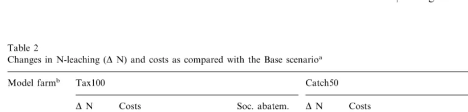
Production type is an important source of variability that Table 1 does not inform us about. Table 2 shows the effects of a tax and a catch crop requirement for a selected group of model farms in Auli. Here we only focus on N-leaching.
In the Base scenario these farms have an average leaching varying between 37 and 42 kg N/ha. MF1 has the lowest and MF4 the highest losses. While the tax has the largest effect on the milk producing model farm, the effect of a 50% catch crops/grass land requirement is negligible here, since it already has nearly 50% of its acreage in grass production. In the case of farms with grain as the dominant crop, the situation is the oppo-site.
We observe a much larger reduction in the use of fertilizer N in grass than in grain production — both absolutely and relatively. While the average effect of a 100% N tax is approximately 27% (40 kg/ha) for grass, the figures for grain are 10% (11 kg/ha). The difference is primarily due to substitu-tion between fertilizer N and clover in producsubstitu-tion of roughage. We observe positive effects following changes in the manuring practices, too. In the case of MF1, Tax100 induces increased storage capacity up till a full year’s storage. This elimi-nates losses related to fall spreading. The greatest effect of this change, however, is due to less compaction damages, hence improved conditions for plant growth.
Finally, we observe that social abatement costs vary rather substantially across the model farms in the case of a 100% tax, while they are much more uniform for the catch crop regime. The private costs are hardest to bear for the special-ized grain farm since per ha incomes are lowest in this case.
5.5. High sensiti6ity for changes in the plant–soil
system
5.5.1. The effect of different tillage practices
The results are, as already observed, heavily dependent upon a series of interacting agronomic factors. One aspect of plant – soil interaction, the effect of tillage practice on N dynamics, caught our interest. Analyzing this more in detail we observed:
Postponing fall tillage by about 5 weeks from the end of August to early October gives, ac-cording to ECECMOD, a reduction in leaching approximately at the level of a 100% N tax in grain dominated areas like Auli and Mørdre. This is entirely an effect of N-uptake by weeds and germinating shed grains and its subsequent influence on the soil micro flora/fauna. The estimates show higher effects in Auli than in Mørdre. This difference relates mostly to the fact that 50% of the area in Mørdre is tilled in spring also in the Base scenario and is thus not influenced by this change. One should take into account that delayed fall tillage induces no extra costs, except the risk that some areas will not be tilled in time in years with rainy au-tumns and/or early frost.
Increased spring tillage (mandatory or follow-ing from a subsidy scheme) turned out, as we have already seen, to give very small effects on N leaching. This was a surprise. Even though the mass of weeds/shed grain is increased by
Table 2
Changes in N-leaching (DN) and costs as compared with the Base scenarioa
Model farmb Tax100 Catch50
Soc. abatem.
DN Costs Soc. abatem. DN Costs
costs kg/ha farmer
kg/ha farmer costs
NOK/kgDN NOK/kgDN
NOK/ha NOK/kgDN NOK/ha NOK/kgDN
−10.5 610 59
MF1 18 −1.3 20 16 16
−3.7 510 139 46 300 16 16
MF4 −18.3
−15.9 300 19 19
650 129
MF7 −5.1 10
aSome model farm estimates, Auli.
expanding the growth period for some extra weeks compared to late fall tillage, we observe that the effect of extra plant uptake is counter-acted by a decline in the subsequent main crop yield on sandy and clayey soils the following season.
To comprehend the sensitivity of the system, recognize that the average leaching in the Base scenario is about 20 – 25% of a total plant uptake of about 150 kg N per ha and year. A change in this uptake of about 3% will, other things being equal, create a potential change in leaching at the level induced by a 100% N tax. On clayey soils like the ones in Auli, yield losses following a transition from fall to spring tillage are at the average level of about 4%, explaining much of the above results.
As mentioned, the modelled effect of delayed autumn tillage on nitrate leaching is attributable to N-assimilation by weeds and germinating shed grains throughout the autumn. This has not been confirmed by direct observations of nitrate leach-ing in field experiments, however. The model as-sumes no extra mineralization of soil organic N by tillage, despite the widespread notion that plowing has such effects. However, this is an assertion for which there is very little evidence. Our modelling has pinpointed that nitrate leach-ing is sensitive to such possible direct effects of plowing and to N-assimilation by weeds and ger-minating shed grains. This puts new questions on the agenda for natural scientists about the specific mechanisms invoked by ploughing, and on the N-assimilation by weeds.
5.5.2. Split fertilization
The assumed positive effect of split fertilization is related to better adjustment of the fertilizer level to the actual growing conditions each year. A more complete analysis of the issue is given in Romstad and Rørstad (1995). Here we will em-phasize the following:
An effect of split fertilizing is lower fertilizer levels in ‘bad’ years, but also increased levels in ‘good’ years. To create an environmentally in-teresting scheme, the total level of N must be reduced even for split fertilizing.
A system combining reduced and split fertiliza-tion can be obtained by a scheme of season-specific tradeable N quotas. Except for sandy soils, the results obtained from such a scheme are not very different from those obtained us-ing a uniform N-tax givus-ing the same reductions in the overall fertilizer levels. The costs for farmers are considerably lower (no taxes), while the administration costs are expected to be higher.
The difference between sandy soils and other soils was as expected. The results for clay and silt were still surprising to us since yields also vary substantially between years in these cases. Interac-tions between hydrology and the biological sink mechanisms explain much of the observed effects. Further, the results depend strongly on the preci-sion of the crop growth modelling. To exemplify: in our analyses, average yield is reduced by ap-proximately 2% due to the extra trafficking fol-lowing a second round N application. As we have already seen, this is of a magnitude influencing leaching rather substantially. The positive effect of increased fertilizing precision obtained by split fertilizing is thus more or less nullified by this seemingly minor effect on the yield for both clayey and silty soils.
6. Conclusion
Adequate understanding of the basis for farm-ers’ choices, both from an agronomic and social science point of view, is important. We have used a profit maximization rule in our analysis, believ-ing that it is an adequate basis for ‘comparbeliev-ing changes’ in adaptation under different policy sce-narios. We admit that it does not offer a complete description of agents’ behavior. Still, progress is obtained by undertaking a detailed description of the setting and constraints under which choices are made. Farmers respond differently to political measures, depending on their production system, warranting a careful economic analysis of such choices at a reasonably high resolution.
The interdisciplinary discourse is necessary to identify and nurture new/more relevant research within each discipline. The division of science into rather narrow subfields has been necessary to increase the depth of the analysis. As the only strategy, however, it prevents the understanding of inter-linkages and dynamics at higher system levels. Practical relevance may be lost. Interdisci-plinary research may serve us greatly by just making the disciplines relate better to higher re-spective lower level entities.
ECECMOD is a structure that can be devel-oped in different directions. First of all other pollution problems like pesticide use can be inte-grated, a process we have started on. Such an enlargement has proven to be relatively easy to undertake without having to make major changes in the system. This is both an effect of the way ECECMOD is structured, its process orientation, and the level of resolution chosen.
Acknowledgements
The project is financed by the Research Council of Norway. The authors would like to thank Halstein Lundeby, Per Kr. Rørstad and Arild Vold for their participation in the development of ECECMOD. We would also like to credit the approximate 40 colleagues at the Agricultural University of Norway, Center of Soil and Envi-ronmental Research, Norwegian Crop Research Institute, Norwegian Institute of Land Inventory and Statistics Norway providing us with data and
different background analysis. Finally, we thank Reidun Aasheim for assistance in preparing the figures and three reviewers for constructive comments.
References
Antle, J.M., Capalbo, S.M., 1993. Integrating economic & physical models for analyzing environmental effects of agricultural policy on nonpoint-source pollution. In: Rus-sell, C.S., Shogren, J.S. (Eds.), Theory, Modeling and Experience in the Management of Nonpoint-Source Pollu-tion. Kluwer, Boston, MA, pp. 155 – 178.
Botterweg, P.F., 1992. European Soil Erosion Model. Winter routines — possible solutions. Economics & Ecology/
RMPA working paper no 10. Agricultural University of Norway, 12 pp. (unpublished).
Botterweg, P.F., 1998. Snowmelt and frozen soils in simulation models. In: Boardman, J., Favis-Mortlock, D. (Eds.), Modelling Soil Erosion by Water. NATO ASI Series, Series I-55. Springer-Verlag, Berlin, pp. 365 – 376. Botterweg, P., Leek, R., Romstad, R., Vatn, A., 1988. The
Eurosem – Gridsem modelling system for erosion analyses under different natural and economic conditions. Ecol. Modelling 108, 115 – 129.
Christensen, B.T., Johnston, A.E., 1997. Soil organic matter and soil quality: lessons learned from long term field experiments at Askov and Rothamstead. In: Gregonich, E.G., Carter, M.R. (Eds.), Soil Quality for Crop Produc-tion. Elsevier, Amsterdam, pp. 399 – 430.
Costanza, R., Wainger, L., Bockstael, N., 1995. Integrated ecological economic systems modelling: theoretical issues and practical applications. In: Milon, J.W., Shogren, J.F. (Eds.), Integrating Economic and Ecological Indicators. Practical Methods for Environmental Policy Analysis. Praeger, Westport, pp. 45 – 66.
Hausman, J.A. (Ed.), 1993. Contingent Valuation. A Critical Assessment. North-Holland, Amsterdam.
Hodgson, G.M., 1988. Economics and Institutions. Polity Press, Cambridge.
Jansson, P.E., 1991. Simulation model for soil water and heat conditions. Description of the SOIL model. Report 165. Swedish University of Agricultural sciences, Department of Soil Sciences, Uppsala.
Johnsson, H., Bergstro¨m, L., Jansson, P.E., Paustian, K., 1987. Simulated nitrogen dynamics and losses in a layered agricultural soil. Agric. Ecosyst. Environ. 18, 333 – 356. Leek, R., 1993. Using Remote Sensing for Terrestrial
Moni-toring and Prediction of Sediment Yield to Rivers. Report no 35, report series Hydrology. University of Norway. Morgan, R.P.C., Quinton, J.N., Smith, R.E., Govers, G.,
Nakajima, C., 1986. Subjective Equilibrium Theory of the Farm Household. Elsevier, Amsterdam.
O’Neill, R.V., DeAngelis, D.L., Waide, J.B., Allen, T.F.H., 1986. A Hierachical Concept of Ecosystems. Princeton University Press, Princeton, NJ.
Rastetter, E.B., King, A.W., Hornberger, G.M., Cosby, B.J., O’Neill, R.V., Hobbie, J.E., 1992. Aggregating fine scale ecological knowledge to model coarse-scale attributes of ecosystems. Ecol. Appl. 2 (1), 55 – 70.
Romstad, E., Rørstad, P.K., 1995. Policy Measures to Induce Split Fertilization in Grain Production, IØS Discussion Paper cD-18/1995, Agricultural University of Norway (unpublished).
Simon, H.A., 1979. Rational decision making in business organization. Am. Econ. Rev. 69 (4), 439 – 513.
Singh, I., Squire, L., Strauss, J., 1986. Agricultural Household Models. Extensions, Applications and Policy. John Hop-kins Press, Baltimore, MD.
Uhlen, G., 1989. Nutrient leaching and surface runoff in field lysimeters on a cultivated soil. Nutrient balances 1974 – 81. Norwegian J. Agric. Sci. 68 (3), 33 – 46.
Vatn, A., Bromley, D.W., 1994. Choices without prices with-out apologies. J. Environ. Econ. Manage. 26, 129 – 148. Vatn, A., Bakken, L., Bleken,. M.A., Botterweg, P., Lundeby,
H., Romstad, E., Rørstad. P.K., Vold, A., 1996. Policies for reduced nutrient losses and erosion from Norwegian agriculture. Integrating economics and ecology. Norwegian J. Agric. Sci., Supplement no 23.
Vatn, A., Bakken, L., Bleken, M.A., Botterweg, P., Lundeby, H., Romstad, E., Rørstad, P.K., Vold, A., 1997. Regulat-ing nonpoint-source pollution from agriculture — an inte-grated modelling analysis. Eur. Rev. Agric. Econ. 24, 207 – 229.
Vedeld, P., 1998. Farmers and Fertilizers. A Study of Adapta-tion and Response to Price Change among Norwegian Farmers. Ph.D.thesis. Department of Economics and So-cial Sciences, Agricultural University of Norway. Vold, A., 1997. Development and evaluation of a
mathemati-cal model for plant N-uptake and N-leaching from agricul-tural soils. Doctor scientiarium thesis 1997:28, Agriculagricul-tural University of Norway.
Vold, A., Breland, T.A., Bakken, L.R., 1994. Prediction of short- and long-term effects of green manuring. In: Linde`n, B. (Ed.), The Use of Catch or Cover Crops to Reduce Leaching and Erosion. NJF-utredning/rapport nr. 99, Proc. NJF-seminar no. 245, pp. 181 – 192.
Vold, A., Bakken, L.R., Vatn, A., 1995. The use of a simu-lated barley cropping system as a bioassay for estimating net effects of catch crop and manure application on the N-availability to subsequent crops. Economics & Ecology/
RMPA Working paper no 40. Agricultural University of Norway, 23 pp. (unpublished).
Vold, A., Bakken, L.R., Uhlen. G., Vatn, A., 1999. Use of data from long term experiments to model plant nitrogen uptake. Nutr. Cycling Agroecosyst., in press.
.