Advanced mathematical methods

(1)

Advanced Mathematical Methods

with Maple

(2)

p u b l i s h e d b y t h e p r e s s s y n d i c a t e o f t h e u n i v e r s i t y o f c a m b r i d g e The Pitt Building, Trumpington Street, Cambridge, United Kingdom

c a m b r i d g e u n i v e r s i t y p r e s s The Edinburgh Building, Cambridge CB2 2RU, UK 40 West 20th Street, New York, NY 10011–4211, USA

10 Stamford Road, Oakleigh, VIC 3166, Australia Ruiz de Alarc ´on 13, 28014 Madrid, Spain

Dock House, The Waterfront, Cape Town 8001, South Africa http://www.cambridge.org

c

Derek Richards 2002

This book is in copyright. Subject to statutory exception and to the provisions of relevant collective licensing agreements,

no reproduction of any part may take place without the written permission of Cambridge University Press.

First published 2002

Printed in the United Kingdom at the University Press, Cambridge

TypefaceTimes 10/13pt. SystemLA_{TEX 2ε} _[uph] A catalogue record for this book is available from the British Library

Library of Congress Cataloguing in Publication data

Richards, Derek.

Advanced mathematical methods with Maple / Derek Richards. p. cm.

Includes bibliographical references and index. ISBN 0 521 77010 6 – ISBN 0 521 77981 2 (pb.)

1. Numerical analysis–Data processing. 2. Maple (Computer file) I. Title. QA297.R495 2001

519.4′_0285–dc21 _{2001025976 CIP}

(3)

7.2.2 Basic properties of the delta function 228 7.2.3 The delta function as a limit of a sequence 232 7.3 Green’s functions: an introduction 238 7.3.1 A digression: two linear differential equations 239 7.3.2 Green’s functions for a boundary value problem 244 7.3.3 The perturbed linear oscillator 248 7.3.4 Numerical investigations of Green’s functions 251 7.3.5 Other representations of Green’s functions 252 7.4 Bessel functions: Kapteyn and Neumann series 254 7.5 Appendix 1: Bessel functions and the inverse square law 258

7.6 Appendix 2: George Green 261

7.7 Exercises 262

8 Fourier series and systems of orthogonal functions 267

8.2 Orthogonal systems of functions 269 8.3 Expansions in terms of orthonormal functions 270

8.4 Complete systems 271

(6)

viii Contents

8.6 Addition and multiplication of Fourier series 276 8.7 The behaviour of Fourier coefficients 277 8.8 Differentiation and integration of Fourier series 280 8.9 Fourier series on arbitrary ranges 284

8.10 Sine and cosine series 284

8.11 The Gibbs phenomenon 286

8.12 Poisson summation formula 291 8.13 Appendix: some common Fourier series 293

8.14 Exercises 293

9 Perturbation theory 301

9.2 Perturbations of algebraic equations 302

9.2.1 Regular perturbations 302

9.2.2 Singular perturbations 305

9.2.3 Use of Maple 308

9.2.4 A cautionary tale: Wilkinson’s polynomial 313

9.3 Iterative methods 315

9.3.1 A nasty equation 319

9.4 Perturbation theory for some differential equations 320 9.5 Newton’s method and its extensions 325 9.5.1 Newton’s method applied to more general equations 328 9.5.2 Power series manipulation 331

9.6 Exercises 336

10 Sturm–Liouville systems 342

10.2 A simple example 343

10.3 Examples of Sturm–Liouville equations 345

10.4 Sturm–Liouville systems 352

10.4.1 On why eigenvalues are bounded below 360

10.5 Green’s functions 361

10.5.1 Eigenfunction expansions 365

10.5.2 Perturbation theory 369

10.6 Asymptotic expansions 371

10.7 Exercises 375

11 Special functions 377

11.2 Orthogonal polynomials 377

11.2.1 Legendre polynomials 381

11.2.2 Tchebychev polynomials 386

11.2.3 Hermite polynomials 389

11.2.4 Laguerre polynomials 395

(7)

Contents ix

11.4 Bessel functions 404

11.5 Mathieu functions 410

11.5.1 An overview 411

11.5.2 Computation of Mathieu functions 416

11.5.3 Perturbation theory 421

11.5.4 Asymptotic expansions 425

11.6 Appendix 429

11.7 Exercises 431

12 Linear systems and Floquet theory 437

12.2 General properties of linear systems 438

12.3 Floquet theory 443

12.3.2 Parametric resonance: the swing 444 12.3.3 O Botafumeiro: parametric pumping in the middle ages 446 12.3.4 One-dimensional linear systems 447 12.3.5 Many-dimensional linear, periodic systems 448

12.4 Hill’s equation 452

12.4.1 Mathieu’s equation 454

12.4.2 The damped Mathieu equation 457

12.5 The Li´enard equation 466

12.6 Hamiltonian systems 467

12.7 Appendix 471

12.8 Exercises 473

13 Integrals and their approximation 478

13.2 Integration with Maple 482

13.2.1 Formal integration 482

13.2.2 Numerical integration 489

13.3 Approximate methods 492

13.3.1 Integration by parts 493 13.3.2 Watson’s lemma and its extensions 497 13.4 The method of steepest descents 506 13.4.1 Steepest descent with end contributions 514

13.5 Global contributions 516

13.6 Double integrals 520

13.7 Exercises 521

14 Stationary phase approximations 526

14.2 Diffraction through a slit 528 14.3 Stationary phase approximation I 532

(8)

x Contents

14.3.2 General first-order theory 539 14.4 Lowest-order approximations for many-dimensional integrals 541 14.5 The short wavelength limit 544

14.6 Neutralisers 545

14.7 Stationary phase approximation II 554

14.7.1 Summary 555

14.8 Coalescing stationary points: uniform approximations 557

14.8.1 Rainbows 557

14.8.2 Uniform approximations 562

14.9 Exercises 569

15 Uniform approximations for differential equations 573

15.2 The primitive WKB approximation 575

15.3 Uniform approximations 579

15.3.1 General theory 579

15.3.2 No turning points 581

15.3.3 Isolated turning points 582 15.4 Parabolic cylinder functions 587 15.4.1 The equation y′′+ (x2/4−a)y= 0 588 15.4.2 The equation y′′−₍x2_/_{4 +}_a₎_y_{= 0} ₅₉₂

15.5 Some eigenvalue problems 594 15.5.1 A double minimum problem 602 15.6 Coalescing turning points 606 15.6.1 Expansion about a minimum 606 15.6.2 Expansion about a maximum 609 15.6.3 The double minimum problem 610

15.6.4 Mathieu’s equation 615

15.7 Conclusions 621

15.8 Exercises 623

16 Dynamical systems I 628

16.2 First-order autonomous systems 634 16.2.1 Fixed points and stability 634

16.2.2 Natural boundaries 637

16.2.3 Rotations 637

16.2.4 The logistic equation 638

16.2.5 Summary 641

16.3 Second-order autonomous systems 641

16.3.2 The phase portrait 644

(9)

Contents xi

16.3.6 The linearisation theorem 664

16.3.7 The Poincar´e index 665

16.4 Appendix: existence and uniqueness theorems 668

16.5 Exercises 669

17 Dynamical systems II: periodic orbits 673

17.2 Existence theorems for periodic solutions 674

17.3 Limit cycles 677

17.3.1 Simple examples 677

17.3.2 Van der Pol’s equation and relaxation oscillations 678 17.4 Centres and integrals of the motion 684

17.5 Conservative systems 691

17.6 Lindstedt’s method for approximating periodic solutions 697 17.6.1 Conservative systems 698

17.6.2 Limit cycles 705

17.7 The harmonic balance method 707 17.8 Appendix: On the Stability of the Solar System,by H. Poincar´e 711 17.9 Appendix: Maple programs for some perturbation schemes 717 17.9.1 Poincar´e’s method for finding an integral of the motion 717 17.9.2 Lindstedt’s method applied to the van der Pol oscillator 719 17.9.3 Harmonic balance method 721

17.10 Exercises 723

18 Discrete Dynamical Systems 727

18.2 First-order maps 728

18.2.1 Fixed points and periodic orbits 728

18.2.2 The logistic map 731

18.2.3 Lyapunov exponents for one-dimensional maps 739 18.2.4 Probability densities 742 18.3 Area-preserving second-order systems 746 18.3.1 Fixed points and stability 746

18.3.2 Periodic orbits 751

18.3.3 Twist maps 753

18.3.4 Symmetry methods 757

18.4 The Poincar´e index for maps 762

18.5 Period doubling 764

18.6 Stable and unstable manifolds 767 18.6.1 Homoclinic points and the homoclinic tangle 772

18.7 Lyapunov exponents 774

18.8 An application to a periodically driven, nonlinear system 776

(10)

xii Contents

19 Periodically driven systems 785

19.1 Introduction: Duffing’s equation 785 19.2 The forced linear oscillator 786 19.3 Unperturbed nonlinear oscillations 789 19.3.1 Conservative motion,F =µ= 0:ǫ <0 789 19.3.2 Conservative motion,F =µ= 0:ǫ >0 793 19.3.3 Damped motion:F= 0,µ >0 796 19.4 Maps and general considerations 797 19.5 Duffing’s equation: forced, no damping 807 19.5.1 Approximations toT-periodic orbits 807

19.5.2 Subharmonic response 813

19.6 Stability of periodic orbits: Floquet theory 815

19.7 Averaging methods 817

19.7.1 Averaging over periodic solutions 817

19.7.2 General theory 819

19.7.3 Averaging over a subharmonic 823 19.8 Appendix: Fourier transforms 825

19.9 Exercises 828

20 Appendix I: The gamma and related functions 834

21 Appendix II: Elliptic functions 839

22 References 845

22.1 References 845

22.2 Books about computer-assisted algebra 853

(11)

8

Fourier series and systems of orthogonal functions

8.1 Introduction

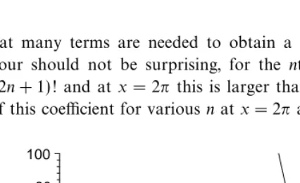
In chapter 4 we introduced Taylor’s series, a representation in which the function is expressed in terms of the value of the function and all its derivatives at the point of expansion. In general such series are useful only close to the point of expansion, and far from here it is usually the case that very many terms of the series are needed to give a good approximation. An example of this behaviour is shown in figure 8.1, where we compare various Taylor polynomials of sinxaboutx= 0 over the range 0< x <2π.

(15)

(11) (9)

–2 –1 0 1 2

1 2 _x 3 4 5 6

Figure 8.1 Taylor polynomials of sinxwith degree 9, 11 and 15.

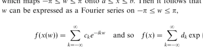
It is seen that many terms are needed to obtain a good approximation at x = 2π. Such behaviour should not be surprising, for the nth term of the Taylor’s series is (₋1)n_x2n+1_/₍₂_n_{+ 1)! and at}_x_{= 2}_π _{this is larger than 1 if}_n

≤6. Some values of the magnitude of this coefficient for variousnat x= 2π and 3πare shown in figure 8.2.

n

π

3

π

2

0 20 40 60 80 100

2 4 6 8 10 12

Figure 8.2 Dependence ofx2n+1_/₍₂_n_{+ 1)!, at}_x_{= 2}_π_{and 3}_π_,

uponn.

(12)

268 Fourier series and systems of orthogonal functions

A Taylor’s series approximation is most accurate near the point of expansion, x=a, and its accuracy generally decreases as _|x₋a_|increases, so this type of approximation suffers from the defect that it is not usually uniformly accurate over the required range of x, although the Pad´e approximant of the Taylor’s series, introduced in chapter 6, can often provide improved accuracy.

Fourier series eliminate these problems by approximating functions in a quite different manner. The essential idea is very simple. Suppose we have a set of functions φk(x),

k = 1,2, . . . , (which may be complex) defined on some interval a _≤ x _≤ b; these could be, for instance, the polynomials φk(x) = xk_{, or the trigonometric functions}

φk(x) = sinkx. Then we attempt to approximate a functionf(x) as the sum

f(x)_≃fN(x) = N X

k=1

ckφk(x)

by choosing the coefficients ck to minimise the mean square difference

EN = Z b

a

dx

f(x)₋ N X

k=1

ckφk(x) 2

.

This is a more democratic method of approximation because no point in the interval is picked out for favoured treatment, as in a Taylor’s series. In order to put this idea into practice we need to know how to choose the functions φk(x) and to understand how the approximation converges with increasing N. For this it is necessary to introduce the notion of a complete set of functions together with some connected technical details.

Exercise 8.1

Use Stirling’s approximation to show that the modulus of thenth term of the Taylor’s series of sinx,x2n+1_/₍₂_n_{+ 1)!, is small for}_{n > ex/}_{2, and that for large}_|_x_|_{the largest term in the}

Taylor’s series has a magnitude of aboutex_/√₂_πx_.

In addition show that with arithmetic accurate toNsignificant figures the series approx-imation for sinxcan be used directly to find values of sinxaccurate toM(< N) significant figures only forx <(N−M) ln 10. Check this behaviour using Maple.

Exercise 8.2

This exercise is about the approximation of sinxon the interval (0, π) using the functions

φ1= 1,φ2=xandφ3=x2.

Use Maple to evaluate the integral

E(a, b, c) =

Z π

0

dx a+bx+cx2−sinx2

to form the function E(a, b, c) which is quadratic in a, bandc. Find the position of the minimum of this function by solving the three equations ∂E

∂a = 0, ∂E

∂b = 0 and ∂E

∂c = 0 fora, bandc. Hence show that

sinx_≃12π

2₋₁₀

π3 −60

π2₋₁₂

(13)

8.2 Orthogonal systems of functions 269

Compare your approximation graphically with the exact function and various Taylor polynomials.

Note that with Maple it is relatively easy to include higher order polynomials in this expansion: it is worth exploring the effect of doing this.

8.2 Orthogonal systems of functions

Here we consider complex functions of the real variable x on an interval a _≤x _≤b. Theinner productof two such functionsf(x) andg(x) is denoted by (f, g) and is defined by the integral

(f, g) = Z b

a

dx f∗(x)g(x), (8.1)

where f∗ _{denotes the complex conjugate of} _f_{; note that (}_{g, f}_{) = (}_{f, g}₎∗_{. The inner} product of a function with itself is real, positive and √(f, f) is named the norm. A function whose norm is unity is said to benormalised.

Two functions f and g are orthogonal if their inner product is zero, (f, g) = 0. A system of normalised functionsφk(x),k= 1,2, . . . ,every pair of which is orthogonal is named anorthogonal system. If, in addition, each function is normalised, so

(φr, φs) =δrs =

1, r=s,

0, r₆=s,

the system is called an orthonormal system. The symbol δrs introduced here is named theKronecker delta. An example of a real orthonormal system on the interval (0,2π), or more generally any interval of length 2π, is the set of functions

1 √

2π,

cosx √

π ,

cos 2x √

π , . . . ,

coskx √

π , . . . .

On the same interval the set of complex functions

φk(x) = e ikx √

2π, k= 0,±1,±2, . . .

is also an orthonormal system.

Exercise 8.3

Find the appropriate value of the constantAthat makes the norm of each of the functions

φ1(x) =Ax, φ2(x) =A(3x2−1), φ3(x) =Ax(5x2−3)

on the intervals−1≤x≤1 and 0≤x≤1, unity. For each interval determine the matrix of inner products (φi, φj) fori, j= 1,2,3.

Exercise 8.4

By evaluating (h, h), whereh(x) = (f, g)f(x)−(f, f)g(x), and using the fact that (h, h)≥0, prove the Schwarz inequality,

(14)

Exercise 8.5

Show that the functions

φk(x) =

are orthogonal on any interval of lengthα.

8.3 Expansions in terms of orthonormal functions

Suppose that φk(x), k= 1,2, . . . , is a system of orthonormal functions on the interval

and choose the N coefficientsck — which may be complex — to minimise the square of the norm of (fN−f). That is, we minimise the function

It follows from this last expression thatF(c) has its only minimum when the first term is made zero by choosing

cj= φj, f, j= 1,2, . . . , N. (8.5)

The numbers cj = (φj, f) are the expansion coefficients of f with respect to the orthogonal system _{φ1, φ2, . . .}. This type of approximation is called anapproximation

in the mean.

An important consequence follows from the trivial observation that

Z b

and by expanding the integrand and integrating term by term to give

(15)

8.4 Complete systems 271

Since (f, f) is independent ofN it follows that

∞ X

k=1

|ck|2≤(f, f), Bessel’s inequality. (8.6)

Bessel’s inequality is true for every orthogonal system: it shows that the sum of squares of the coefficients always converges, provided the norm offexists. From this inequality it follows from section 4.3.1 thatck →0 ask→ ∞.

Exercise 8.6 Derive equation 8.4.

Exercise 8.7

Equations 8.5, for the expansion coefficients, and Bessel’s inequality, equation 8.6, were both derived for an orthonormal system for which (φj, φk) =δjk. Show that if theφk are

orthogonal, but not necessarily orthonormal, these relations become

cj=

(φj, f)

(φj, φj)

and

∞ X

k=1

|(φk, f)|2

(φk, φk) ≤

(f, f).

8.4 Complete systems

Acomplete orthogonal system, φk(x), k= 1,2, . . . , has the property that any function, taken from a given particular set of functions, can be approximated in the mean to any desired accuracy by choosingN large enough. In other words, for any ǫ >0, no matter how small, we can find anN(ǫ) such that forM > N(ǫ)

Z b

a

dx

f(x)− M X

k=1

ckφk(x) 2

< ǫ, where ck= (φk, f) (φk, φk)

. (8.7)

That is, the mean square error can be made arbitrarily small. Notice that this definition needs the functionf to belong to a given set, normally the set of integrable functions. For a complete orthogonal system it can be proved that Bessel’s inequality becomes the equality

(f, f) = ∞ X

k=1

(φk, φk)|ck|2= ∞ X

k=1

(φk, f)2 (φk, φk)

, (8.8)

and this is known as thecompleteness relation. It may also be shown that a sufficient condition for an orthogonal system to be complete is that this completeness relation holds; a proof of this statement is given in Courant and Hilbert (1965, page 52).

There are three points worthy of note.

(16)

• Second, the fact that

lim N→∞

Z b

a

dx

f(x)₋ N X

k=1

ckφk(x) 2

= 0, ck= (φk, f) (φk, φk)

, (8.9)

doesnotimply pointwise convergence, that is,

lim N→∞

N X

k=1

ckφk(x) =f(x), a≤x≤b. (8.10)

If the limit 8.9 holds we say that the sequence of functions

fN(x) = N X

k=1

ckφk(x)

converge to f(x) in the mean. If the limit 8.10 holds fN(x) converges pointwise to

f(x), section 4.6. If, however, the seriesfN(x) converges uniformly then convergence in the mean implies pointwise convergence.

• Third, if two piecewise continuous functions have the same expansion coefficients with respect to a complete system of functions then it may be shown that they are identical, see for example Courant and Hilbert (1965, page 54).

Finally, we note that systems of functions can be complete even if they are not orthogonal. Examples of such complete systems are the polynomialsφk(x) =xk_,

1, x, x2, . . . , xn, . . . ,

which form a complete system in any closed interval a_≤x_≤b, for the approximation theorem of Weierstrass states that any function continuous in the interval a _≤x_≤b

may be approximated uniformly by polynomials in this interval. This theorem asserts uniform convergence, not just convergence in the mean, but restricts the class of functions to be continuous. A proof may be found in Powell (1981, chapter 6).

Another set of functions is 1

x+λ1

, 1

x+λ2

, . . . , 1 x+λn

, . . . ,

where λ1, λ2, . . . , λn, . . .are positive numbers which tend to infinity with increasing n; this set is complete in every finite positive interval. An example of the use of these functions is given in exercise 8.28 (page 294), and another set of complete functions is given in exercise 8.41 (page 298).

In this and the preceding sections we have introduced the ideas of:

• inner product and norm; • orthogonal functions;

• complete orthonormal systems.

(17)

8.5 Fourier series 273

8.5 Fourier series

In modern mathematics a Fourier series is an expansion of a function in terms of a set of complete functions. Originally and in many modern texts the same name is used in the more restrictive sense to mean an expansion in terms of the trigonometric functions

1,cosx,sinx,cos 2x,sin 2x, . . . ,cosnx,sinnx, . . . (8.11)

or their complex equivalents

φk=e−ikx, k= 0,±1,±2, . . . , (8.12)

which are complete and orthogonal on the interval (₋π, π), or any interval of length 2π; the interval (0,2π) is often used. Series of this type are namedtrigonometric series

if it is necessary to distinguish them from more general Fourier series: in the remainder of this chapter we treat the two names as synonyms. Trigonometric series are one of the simplest of this class of Fourier expansions — because they involve the well understood trigonometric functions — and have very many applications.

Any sufficiently well behaved functionf(x) may be approximated by thetrigonometric series

F(x) = ∞ X

k=−∞

cke−ikx, ck= (φk, f) (φk, φk)

= 1 2π

Z π

−π

dx eikxf(x), (8.13)

where we have used the first result of exercise 8.7. We restrict our attention to real functions, in which casec0is real, and is just the mean value of the functionf(x), and

c₋k=c∗k. The constantsck are named theFourier coefficients. The Fourier seriesF(x) is often written in the real form

F(x) =1 2a0+

∞ X

k=1

akcoskx+ ∞ X

k=1

bksinkx, (8.14)

whereak= 2ℜ(ck), bk= 2ℑ(ck), or

a0= 1

π Z π

−π

dx f(x),

ak

bk

= 1

π Z π

−π

dx

coskx

sinkx

f(x), k= 1,2, . . . . (8.15)

The constantsak and bk are also called Fourier coefficients. It is often more efficient and elegant to use the complex form of the Fourier series, though in special cases, see for instance exercise 8.10, the real form is more convenient.

One of the main questions to be settled is how the Fourier seriesF(x) relates to the original functionf(x). This relation is given by Fourier’s theorem, discussed next, but before you read this it will be helpful to do the following two exercises.

Exercise 8.8

Show that the Fourier series of the functionf(x) =_|x_|on the interval₋π_≤x_≤πis

F(x) = π

2− 4

π

∞ X

k=1

cos(2k₋1)x

(2k−1)2 .

Use Maple to compare graphically theNth partial sum,FN(x), of the above series withf(x)

(18)

Further, show that the mean square error, defined in equation 8.7, of the Nth partial sum decreases asN−3_{. Show also that}

FN(0) =

1

πN +O(N

−2₎_.

In this example we notice that even the first two terms of the Fourier series provide a reasonable approximation to|x_|for−π_≤x_≤π, and for larger values ofNthe graphs ofFN(x) and|x|are indistinguishable over most of the range. A close inspection of the graphs near x= 0, wheref has no derivative, shows that here more terms are needed to obtain the same degree of accuracy as elsewhere.

For _|x_|> π, f(x) and F(x) are different. This is not surprising as F(x) is a periodic function with period π — generally this type of Fourier series is 2π-periodic but here

F(x) is even aboutx=π.

Finally, note that for largek the Fourier coefficientsck areO(k−2); we shall see that this behaviour is partly due to f(x) being even aboutx= 0.

Now consider a function which is piecewise smooth on (−π, π) and discontinuous at

x= 0.

Exercise 8.9

Show that the Fourier series of the function

f(x) =

x/π, −π < x <0,

1−x/π, 0≤x < π,

is

F(x) = 4

π2

∞ X

k=1

cos(2k−1)x

(2k₋1)2 +

2

π

∞ X

k=1

sin(2k−1)x

2k₋1 .

Use Maple to compare graphically theNth partial sum of this series withf(x) forN= 1,4,

10 and 20. Make your comparisons over the interval (₋2π,2π) and investigate the behaviour of the partial sums of the Fourier series in the range₋0.1< x <0.1 in more detail.

Find the values off(0) andf(_±π) and show that

F(0) =1

2 and F(±π) =− 1 2.

Hint: remember that the piecewise function can be defined in Maple using the command

x->piecewise(x<0, x/Pi, 1-x/Pi);.

In this comparison there are four points to notice:

• First, observe that for ₋π < x < π, but x not too near 0 or _±π, FN(x) is close to

f(x) but thatF(x)=6 f(x) atx= 0 and ±π.

• Second, as in the previous example, F and f are different for_|x_|> π becauseF(x) is a periodic extension of f(x).

• Third, in this case the convergence of the partial sums tof(x) is slower because now

ck=O(k−1); again this behaviour is due to the nature off(x), as will be seen later. • Finally, we see that for x _≃ 0, FN(x) oscillates about f(x) with a period that

(19)

8.5 Fourier series 275

Some of the observations made above are summarised in the following theorem, which gives sufficient conditions for the Fourier series of a function to coincide with the function.

Fourier’s theorem

Let f(x) be a function given on the interval ₋π _≤x < π and defined for all other values ofxby the equation

f(x+ 2π) =f(x)

so thatf(x) is 2π-periodic. Assume thatRπ

−πdx f(x) exists and that the complex Fourier coefficientsck are defined by the equations

ck= 1 2π

Z π

−π

dx f(x)eikx, k= 0,_±1, _±2, . . . ,

then if₋π < a_≤x_≤b < π and if in this interval_|f(x)_|is bounded, the series

F(x) = ∞ X

k=−∞

cke−ikx (8.16)

is convergent and has the value

F(x) = 1 2

lim ǫ→0+

f(x+ǫ) + lim ǫ→0+

f(x₋ǫ)

. (8.17)

Iff(x) is continuous at a pointx=wthe limit reduces toF(w) =f(w).

The conditions assumed here are normally met by functions found in practical appli-cations. In the example treated in exercise 8.9 we have, atx= 0,

lim ǫ→0+

f(ǫ) = 1 and lim ǫ→0+

f(−ǫ) = 0,

so equation 8.17 shows that the Fourier series converges to 1

2 atx= 0, as found in the exercise.

Fourier’s theorem gives the general relation between the Fourier series andf(x). In addition it can be shown that if the Fourier coefficients have bounded variation and |ck| →0 ask→ ∞ the Fourier series converges uniformly in the interval 0<|x|< π. Atx= 0 care is sometimes needed as the real and imaginary parts of the series behave differently; convergence of the real part depends upon the convergence of the sum

c0+c1+c2+· · ·, whereas the imaginary part is zero, sincec0 is real for real functions (Zygmund, 1990, chapter 1).

The completeness relation, equation 8.8 (page 271), modified slightly because the functions used here are not normalised, gives the identity

∞ X

k=−∞

|ck|2= 1 2π

Z π

−π

dx f(x)2, (8.18)

or, for the real form of the Fourier series,

1 2a

2 0+

∞ X

k=1

a2_k+b2_k = 1

π Z π

−π

(20)

These relations are known as Parseval’s theorem. It follows from this relation that if the integral exists_|ck|tends to zero faster than|k|−1/2 as|k| → ∞.

There is also a converse of Parseval’s theroem: the Riesz–Fischer theorem, which states that if numbers ck exist such that the sum in equation 8.18 exists then the series defined in equation 8.13 (page 273), is the Fourier series of a square integrable function. A proof of this theorem can be found in Zygmund (1990, chapter 4).

In the appendix to this chapter some common Fourier series are listed.

Exercise 8.10

Show that iff(x) is a real function even aboutx= 0 then its Fourier series, on the interval (−π, π), contains only cosine terms, but that if f(x) is an odd function its Fourier series contains only sine terms.

Exercise 8.11

LetF(x) be the Fourier series of the functionf(x) =x2 _{on the interval 0}_≤_x_≤₂_π_{. Sketch}

the graph ofF(x) in the interval (−2π,4π). What are the values ofF(2nπ) for integern? Note, you are not expected to find an explicit form forF(x).

Exercise 8.12

Observe that forr <1 the Fourier coefficients tend to zero faster than exponentially with increasing k, in contrast to the Fourier coefficients obtained in exercises 8.8 and 8.9, for example.

8.6 Addition and multiplication of Fourier series

The Fourier coefficients of the sum and difference of two functions are given by the sum and difference of the constituent coefficients, as would be expected. Thus if

(21)

8.7 The behaviour of Fourier coefficients 277

then, for any constantsaandb,

af1(x) +bf2(x) = ∞ X

k=−∞

(ack+bdk)e−ikx.

The Fourier series of the product of the two functions is, however, more complicated; suppose that

f1(x)f2(x) = ∞ X

k=−∞

Dke−ikx, (8.21)

then if the Fourier series forf1 andf2 are absolutely convergent we also have

f1(x)f2(x) = ∞ X

k=−∞ ∞ X

l=−∞

ckdle−i(k+l)x,

= ∞ X

p=−∞

e−ipx

∞ X

k=−∞

ckdp−k. (8.22)

On comparing equations 8.21 and 8.22 we see that the nth Fourier coefficient of the product is

Dn= ∞ X

k=−∞

ckdn−k= ∞ X

k=−∞

cn−kdk. (8.23)

Exercise 8.13

Show that thenth Fourier coefficient of f1(x)2, where the Fourier series off1 is given in

equation 8.20, is

∞ X

k=−∞

ckcn−k.

Use the Fourier series forxto deduce that

∞ X

k=−∞ k6= 0, n

1

k(k₋n) = 2

n2.

Another consequence of equation 8.22 is the addition formula for Bessel functions, exercise 8.31 (page 295).

8.7 The behaviour of Fourier coefficients

(22)

Consider a function havingNcontinuous derivatives on (₋π, π). The integral for the Fourier components, equation 8.13 (page 273), can be integrated by partsNtimes; the first two integrations give

ck =

Clearly this process can be continued until theNth differential appears in the integral, but useful information can be gleaned from these expressions.

Iff(x) is even,f(π) =f(₋π) and it follows thatck=O(k−2). The same result holds if f is not even but f(π) = f(₋π). If the function is odd then ck = O(k−1), unless

f(π) = 0.

If f(x) is 2π-periodic then f(r)(π) = f(r)(₋π), r = 0, 1, . . . , N, and after further integration by parts we obtain

ck = 1

since all the boundary terms are now zero. But

One important consequence of this last result is that the numerical estimate of the mean of a sufficiently well behaved periodic function over a period obtained using N

equally spaced points converges faster than any power ofN−1; this is faster than most other numerical procedures. We prove this using the Fourier series of the function: suppose, for simplicity, that the function is 2π-periodic so possesses the Fourier series

f(x) = ∞ X

k=−∞

Cke−ikx,

where the coefficients Ck are unknown and C0 is the required mean value of f(x). The mean of f(x) over (0,2π) can be approximated by the sum overN equally spaced

Using the Fourier series off(x) the sum can be written in the alternative form

(23)

8.7 The behaviour of Fourier coefficients 279

But we have the relation

N

which follows because the left hand side is a geometric series. Nowz= 2πk/N, and

R find the value ofRby taking the limit, or more easily by noting that the original sum becomes of (Np)−1_{, so that the numerical estimate of the mean on the left hand side converges} toC0 faster than any power ofN−1. This result is of practical value.

The ideas presented in this section can sometimes be put to good use in speeding the convergence of Fourier series. Consider a functionf(x) continuous on−π < x_≤π

but withf(π)₆=f(₋π), so its Fourier coefficientsck=O(k−1), as k→ ∞. Define a new functiong(x) =f(x)−αxwith the constantαchosen to makeg(π) =g(−π), that is

α= 1

2π(f(π)−f(−π)),

so Fourier components ofg behave asO(k−2_).

As an example consider the odd functionf(x) = sin√2xwith the Fourier series

(24)

Hence for₋π_≤x_≤π we may write

f(x) = sin√2x= x

πsinπ √

2 + 4

πsinπ √

2 ∞ X

k=1

(₋1)k−1

k(k2₋₂₎sinkx. (8.28)

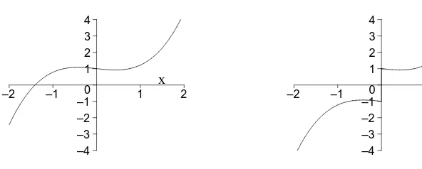
In the following two figures we compare the function,f(x) = sin√2x, with ten terms of the original Fourier series 8.27, on the left, and just two terms of the modified series 8.28, on the right; in the second case with more terms the two functions are practically indistinguishable. The main point to notice is that by removing the discon-tinuity in the Fourier series at x =_±π a far more rapidly converging approximation has been obtained that also convergespointwise over the whole range.

It is clear that further corrections that produce a more rapidly converging Fourier series may be added. This idea is developed further by Lanczos (1966, section 16).

–1 –0.75 –0.5 –0.25 0 0.25 0.5 0.75 1

0.5 1 1.5 x 2 2.5 3

Figure 8.3 Comparison off(x) with ten terms of the original Fourier series 8.27.

–1 –0.75 –0.5 –0.25 0 0.25 0.5 0.75 1

0.5 1 1.5 x 2 2.5 3

Figure 8.4 Comparison off(x) with two terms of the modified Fourier series 8.28.

Exercise 8.14

Show that the Fourier series off(x) = sinhxon (−π, π) is

sinhx=2 sinhπ

π

∞ X

k=1

(−1)k−1_k

1 +k2 sinkx.

Show further that

sinhx=x

πsinhπ−2

sinhπ π

∞ X

k=1

(−1)k−1 k(1 +k2₎sinkx.

Use Maple to compare various partial sums of these two series with sinhx and hence demonstrate that the latter is a more useful approximation.

8.8 Differentiation and integration of Fourier series

(25)

8.8 Differentiation and integration of Fourier series 281

is uniformly convergent fora_≤x_≤b,then

df

and the integral is

Z

whereA is the constant of integration and the sum does not include the k= 0 term. The expressions for the differential and integral of a function given above are not entirely satisfactory: the series forR

dx f(x) is not a Fourier series, and ifck =O(k−1) ask _{→ ∞}the convergence of the series given for f′₍_x_{) is problematical and the series} is certainly not useful.

Integration

The first difficulty may be cured by forming a definite integral and using the known Fourier series forx. The definite integral is

Z x

Substituting this expression forxgives

Z x

Iff(x) is real the alternative, real, form for the integral is

(26)

Exercise 8.15

Use equation 8.32 to integrate the Fourier series forxto show that

x2₌π2

3 −4

∞ X

k=1

(₋1)k−1_cos_kx

k2 .

Explain why the Fourier series for x on (−π, π) depends only on sine functions and that forx2 _{only upon cosine functions.}

Differentiation

For many differentiable functions the leading term in the asymptotic expansion ofck is

O(k−1_{); the reason for this is given in the previous section, particularly equation 8.24.} Then the convergence of the series 8.30 forf′₍_x_{) is questionable even though}_f′₍_x_{) may} have a Fourier series expansion. Normally ck =O(k−1) because the periodic extension of f(x) is discontinuous at x = _±π, then we expect the Fourier coefficients of f′₍_x₎ to also be O(k−1), not O(1) as suggested by equation 8.30. We now show how this is achieved.

The analysis of section 8.7 leads us to assume that for large k

ck= (−1)k

c_∞ k +O(k

−2₎_, _c ∞= ₂1

πi(f(π)−f(−π)),

so we define a constantcby the limit

c= lim k→∞(−1)

k_kc k

and consider the Fourier series

g(x) =−i

∞ X

k=−∞

kck−(−1)kce−ikx

which is clearly related to the series 8.30. With the assumed behaviour ofck, the Fourier components of this series areO(k−1). Now integrate this function using equation 8.31:

Z x

0

du g(u) =f(x)−2 ∞ X

k=1 1

kℜ(kck−(−1)

k_c₎_.

Thus g(x) =f′(x) and we have found the Fourier series off′(x) that converges at the same rate as the Fourier series off(x), that is

df

dx=g(x) =−i

∞ X

k=−∞

kck−(−1)kce−ikx. (8.33)

Iff(x) is real,ℜ(c) = 0 and the real form of the Fourier series is

df dx =−

b

2 + ∞ X

k=1

(kbk−(−1)kb) coskx−kaksinkx ,

whereb=₋2ic= limk_→∞(₋1)k_kb

(27)

8.8 Differentiation and integration of Fourier series 283

Exercise 8.16

Using the Fourier series

x3= 2

∞ X

k=1

(₋1)k−1k2π2−6

k3 sinkx, |x|< π,

and the above expression for the differential of a Fourier series, show that

x2₌π2

3 −4

∞ X

k=1

(−1)k−1

k2 coskx, |x| ≤π.

Explain why the Fourier coefficients forx3 _and_x2 _{are respectively}_O₍_k−1_{) and}_O₍_k−2_{) as}

k→ ∞.

Exercise 8.17 Consider the function

f(x) =

∞ X

k=2

(₋1)k k

k2₋₁sinkx=

i

2

X

|k|≥2

(₋1)k k k2₋₁e−

ikx_.

Show that the Fourier series off′₍_x_{) is}

f′(x) =₋1

2+ cosx+

∞ X

k=2

(₋1)kcoskx k2₋₁.

Find also the series forf′′₍_x_{) and hence show that}_f₍_x_{) =} 1 4sinx+

1 2xcosx.

Exercise 8.18

(i) Iff(x) =eax_{, use the fact that}_f′₍_x_{) =}_af₍_x_{) together with equation 8.33 to show that the}

Fourier coefficients off(x) on the interval (₋π, π) are

ck=

i(₋1)k_c

a+ik

for some numberc.

Show directly that the mean off′₍_x_{) is (}_f₍_π₎₋_f₍₋_π₎₎_/₂_π_{and use this to determine the}

value ofc, hence showing that

eax₌sinhπa

π

∞ X

k=−∞

(−1)k

a+ike

−ikx_.

(ii) By observing thate2ax₌_eax_eax_{, or otherwise, use the Fourier series for}_eax_{to show that}

1 + 2a2

∞ X

k=1

1

a2₊_k2 =

πa

tanhπa,

and by considering the smallaexpansion deduce that, for some numbersfn, ∞

X

k=1

1

k2n =fnπ

(28)

8.9 Fourier series on arbitrary ranges

The Fourier series of a function f(x) over a rangea_≤x_≤b, different from (₋π, π), is obtained using the preceding results and by defining a new variable

w= 2π

b₋a

x₋b+a

2

, x= b+a

2 +

b₋a

2π w, (8.34)

which maps−π_≤w_≤π ontoa_≤x_≤b. Then it follows that the functionf(x(w)) of

w can be expressed as a Fourier series on₋π_≤w_≤π,

f(x(w)) = ∞ X

k=−∞

cke−ikw and so f(x) = ∞ X

k=−∞

dkexp

−i 2πk b₋ax

,

where

dk = 1

b₋a Z b

a

dx f(x) exp ₂

πik b₋ax

, (8.35)

this last relation following from the definition of ck and the transformation 8.34.

Exercise 8.19

Show that the Fourier series off(x) = coshxon the interval (−L, L) is

coshx=sinhL

L 1 + 2

∞ X

k=1

(₋1)k_L2 L2₊_π2_k2 cos

πkx L

!

, ₋L_≤x_≤L.

From the form of this Fourier series we observe that the Fourier components are small only ifk≫L; thus ifLis large many terms of the series are needed to provide an accurate approximation, as may be seen by comparing graphs of partial sums of the series with

coshxon₋L < x < Lfor various values ofL.

8.10 Sine and cosine series

Fourier series of even functions,f(x) =f(−x), comprise only cosine terms, and Fourier series of odd functions,f(x) =₋f(₋x), comprise only sine terms. This fact can be used to produce cosine or sine series ofanyfunction over a given range which we shall take to be (0, π).

For any function f(x) an odd extension,fo(x), may be produced as follows:

fo(x) =

−f(−x), x <0, f(x), x_≥0.

(29)

8.10 Sine and cosine series 285

x

–4 –3 –2 –1 0 1 2 3 4

–2 –1 1 2

Figure 8.5 Original function.

x

–4 –3 –2 –1 0 1 2 3 4

–2 –1 1 2

Figure 8.6 Odd extension.

We would normally use this extension when f(0) = 0 so that fo(x) is continuous at

x= 0. Then the Fourier series of fo(x) on (₋π, π) contains only sine functions and we have, from equation 8.15,

f(x) = ∞ X

k=1

bksinkx, 0< x≤π, with bk= 2

π Z π

0

dx f(x) sinkx, k= 1,2, . . . ,

the latter relation following from equation 8.13. This series is often called thehalf-range Fourier sine series.

Similarly we can extendf(x) to produce an even function,

fe(x) =

f(₋x), x <0, f(x), x_≥0,

an example of which is shown in figure 8.8.

x

–4 –3 –2 –1 0 1 2 3 4

–2 –1 1 2

Figure 8.7 Original function.

x

1 2 3 4

–2 –1 1 2

Figure 8.8 Even extension.

The even extension produces a Fourier series containing only cosine functions, to give thehalf-range Fourier cosine series

f(x) = 1 2a0+

∞ X

k=1

akcoskx, 0< x≤π,

where

ak = 2

π Z π

0

(30)

Exercise 8.20 Show that

x= 2

∞ X

k=1

(₋1)k−1

k sinkx, 0≤x < π,

and

x=π

2 − 4

π

∞ X

k=1

cos(2k−1)x

(2k−1)2 , 0≤x≤π.

Explain why the even extension converges more rapidly.

Use Maple to compare, graphically, the partial sums of these two approximations with the exact function.

Exercise 8.21 Show that

sinx= 4

π

(

1 2−

∞ X

k=1

cos 2kx

4k2₋₁ )

, 0_≤x≤π,

and deduce that

∞ X

k=1

(−1)k−1

4k2₋₁ = π

4− 1 2.

8.11 The Gibbs phenomenon

The Gibbs phenomenon occurs in the Fourier series of any discontinuous function, such as that considered in exercise 8.9, but before discussing the mathematics behind this strange behaviour we give the following description of its discovery, taken from Lanczos (1966, section 10).

The American physicist Michelson_†invented many physical instruments of very high precision. In 1898 he constructed a harmonic analyser that could compute the first 80 Fourier components of a function described numerically; this machine could also construct the graph of a function from the Fourier components, thus providing a check on the operation of the machine because, having obtained the Fourier components from a given function, it could be reconstructed and compared with the original. Michelson found that in most cases the input and synthesised functions agreed well.

† A. A. Michelson (1852–1931) was born in Prussia. He moved to the USA when two years old and is best known for his accurate measurements of the speed of light, which was his life long passion; in 1881 he determined this to be 186 329 miles/sec and in his last experiment, finished after his death, obtained 186 280 miles/sec, the current value for the speed of light in a vacuum is 186 282.397 miles/sec (2.997 924 58×108_{m/sec). In 1887, together with Morley, he published results showing that there was no}