Comparison of scales of climate and soil data for
aggregating simulated yields of winter wheat in Denmark
J.E. Olesen
a,∗, P.K. Bøcher
b, T. Jensen
baDepartment of Crop Physiology and Soil Science, Danish Institute of Agricultural Sciences, PO Box 50, DK-8830 Tjele, Denmark bDepartment of Agricultural Systems, Danish Institute of Agricultural Sciences, PO Box 50, DK-8830 Tjele, Denmark
Abstract
Crop growth models are essentially site-based, and use of such models for assessing regional productivity of crops requires methods for aggregating over space. Different method for aggregating simulated county and national crop yields for winter wheat (Triticum aestivum L.) in Denmark were tested using a crop simulation model (CLIMCROP), which was run with and without irrigation for a range of soil types and climatic conditions. The aggregated county or national yield was calculated by summing simulated yield of each category multiplied by the area, they represent. Ten different combinations of scales of climate and soil data were used. The wheat area was distributed between the different soil types using either a uniform distribution or a distribution that gave preference to soils with high water-holding capacity. The simulated results were compared with Danish county and national yield statistics for winter wheat from the period 1971–1997. There was, in general, a poor relationship between simulated and observed yields when the observed yields had been detrended to remove the technology effect. A larger fraction of the inter-annual variability was captured by the model on the loamy soils compared with the sandy soils. The model was able to capture most of the spatial variation in observed yields, except at the coarsest resolutions of the soil data. The finest resolution of soil and climate data gave a better fit of simulated to observed spatial autocorrelation in yield. The results indicate that upscaling of simulated productivity of crops for Danish conditions requires a spatial resolution of soil data of 10×10 km2or finer. A single climate station may be sufficient if only national yields are estimated, but more stations are required, if regional yields are to be estimated. Consideration should also be given to the distribution of crop area on the different soil types. © 2000 Elsevier Science B.V. All rights reserved.
Keywords: Climate change; Climate sensitivity; Land use; Crop model; Spatial scale; Yield forecasting
1. Introduction
Many impact studies have analysed the effect of changes of climatic variables and of atmospheric CO2
concentration on crop production. Most studies have used simulation models applied at individual sites (e.g., Semenov et al., 1996; Brown and Rosenberg, 1997) or in grid boxes across smaller or larger areas
∗Corresponding author. Tel.:+45-89991659; fax:+45-89991619.
E-mail address: [email protected] (J.E. Olesen).
(e.g., Harrison and Butterfield, 1996; Davies et al., 1997; Dhakhwa et al., 1997). These crop models are designed to be run at specific sites with specific soil and climate characteristics.
Current crop models have been shown to only ex-plain a small proportion of the variation in winter wheat (Triticum aestivum L.) yields in UK and Den-mark (Landau et al., 1998; Olesen et al., 2000). The weather in UK and Denmark is generally favourable for cereal crops, and observed regional yields can be as high as 9 Mg ha−1. The yield variation is
there-fore not mainly caused by direct effects of weather on
crop physiology, but by secondary effects such as the presence and effects of weeds, pests, diseases, lodging and anaerobic soil conditions (Jamieson et al., 1999). These effects are not handled by current crop models, and some of them interact strongly with both weather and crop management.
The area grown with winter wheat in Denmark increased sevenfold from 1971 to 1997. The increase in wheat area occurred at the expense of the area with spring barley (Hordeum vulgare L.). The in-crease in winter wheat area can largely be attributed to higher-yielding varieties (Silvey, 1994) and the in-troduction of effective fungicides for disease control (Orson, 1995). The relative increase in wheat area was largest in the counties with sandy soils, indicating that winter wheat has expanded onto lighter soils with lower soil water-holding capacities. This change in land allocation may have influenced the response of national yields to weather, because of different yield responses on different soil types (Wassenaar et al., 1999; Olesen et al., 2000).
Only little attention has been given to the problem of scaling simulated crop production across areas of contrasting soils and climate (LeDuc and Holt, 1987; Easterling et al., 1998; Wassenaar et al., 1999). This upscaling is necessary in order to obtain esti-mates of crop production at aggregated regional or national levels. The aggregated yield is the weighted sum of yields obtained under different climatic, soils and management conditions. The interaction between these factors and the correlation of yields over space affect the aggregated yield variability. Simulated site yields in Denmark have been shown to respond dif-ferently to climatic variation on different soil types (Olesen et al., 2000), which would make the re-sponse of aggregated yield strongly dependent on the soil×climate interaction. Other factors operating at higher scales may, however, be linked with soils and climate variation, and influence actual aggregated yields, e.g., farm types and land use restrictions. The optimal scales of climate and soil data for estimat-ing county and national yields can thus not be easily deduced.
The purpose of this study was to examine the effects of different scales of climate and soil data on simulated yield of winter wheat on regional and national scales in Denmark, and to compare these simulated aggregated yields with observed yields.
2. Materials and methods
The methodology used for upscaling simulated win-ter wheat yield response to climate variability involves three steps. First the necessary soil, climate and land use data are transformed to the required spatial reso-lution. Secondly the crop simulation model is used to calculate yield with and without irrigation for all rel-evant combinations of soils and climate. Finally the output is aggregated to either county or national level by weighing simulated yields according to the area represented by each simulation run.
Various scales of climate and soil data have been compared. These data have three components: cli-mate data (excluding precipitation), precipitation data and soil data. Each scale is given a three-letter name denoting each of these components (e.g., 1RP), see Table 1. Only 10 of the 18 possible combinations of scales were evaluated, omitting the combinations of spatially detailed climate data with spatially coarse soil data. The selected combinations allowed the ef-fect of spatial scale of climate data to be evaluated at the finest spatial resolution of soil data, whereas the spatial scale of soil data was evaluated at two spatial scales of climate data. The actual allocation of wheat on different soil types is not known. The comparison of scales of input data was therefore performed for two different ways of distributing wheat area onto the soil types within each county. One method assumed a uniform distribution of wheat across all soil types. The other method gave preference to soils with high water-holding capacity.
2.1. Crop model
The CLIMCROP model describes the effects of cli-mate on crop production and yield of winter wheat (Olesen et al., 2000). The model includes a crop model and a soil model that is updated in daily time steps.
Table 1
Denomination of the spatial scales of climate and soil data Index Description
Climate data (excluding precipitation)
1 One climate station only (Ødum)
6 Six climate stations with spatial representation according to a maximum correlation scheme Precipitation data
O Precipitation data from each (1 or 6) climate station used directly
R Precipitation data from each (1 or 6) climate station scaled to the precipitation ratio applicable for each 1×1 km2 grid
G Precipitation data from all (650) Danish stations interpolated onto a 10×10 km2grid Soil data
P Data on top and subsoil types taken from the Danish soil survey at its finest spatial resolution G The most representative top and subsoil type within each 10×10 km2 grid cell
C The most representative top and subsoil type within each county
The phenology submodel is identical to that of the SIRIUS wheat model (Jamieson et al., 1998) with a few exceptions (Olesen et al., 2000). The leaf area growth from emergence to 1 March is described as a linear function of soil temperature sum. The devel-opment of green leaf area index during the growing season is described by a logistic equation in soil or air thermal time prior to start of senescence. From this point green leaf area index declines linearly with thermal time. The rate of leaf area expansion during the growing season is affected by winter survival through an effect of daily soil minimum temperature (Olesen et al., 2000).
Nitrogen supply is the main factor controlling crop growth and yield of winter cereals under the humid temperate conditions of northern Europe (Asseng et al., 2000). The optimal nitrogen fertilisation to win-ter wheat crops varies from 124 kg N ha−1 on sandy
soils to 180 kg N ha−1on loamy soils (Knudsen et al.,
1997). The maximum leaf area index has in many studies been found to be proportional to nitrogen up-take (e.g., van Keulen and Stol, 1991; Grindlay, 1997; Sylvester-Bradley et al., 1997). The model uses a maximum leaf area index of 5 on loamy soils (Olesen et al., 2000). The observed variation in optimal nitro-gen fertilisation would thus imply a maximum leaf area index of 3.4 on the sandy soils, given that nitro-gen use efficiencies were identical across soil types.
The leaf area parameters in the model were there-fore adjusted depending on soil type and irrigation management in accordance with Danish nitrogen fertiliser recommendations for different soil types (Plantedirektoratet, 1997). Both leaf area expansion
rate and maximum leaf area index were reduced by 40% under unirrigated conditions on soil types 1 and 2, and on soil type 3 with a sandy subsoil. For soil type 7 and soil type 3 with a clayey subsoil the reduc-tion was set to 20%. The reducreduc-tion was set to 20% on soil types 1–3 (Table 3).
Dry matter production is calculated using a radia-tion use efficiency which is restricted by low tempe-ratures and reduced transpiration (Aslyng and Hansen, 1982).
The sowing date was set to 15 September in all si-mulation runs, because a sensitivity analysis had shown that the simulated effects of a realistic varia-tion in sowing date on yield was small under current climatic conditions in Denmark (Olesen et al., 2000). The crop is harvested at physiological maturity, and yield is based on 15% grain moisture.
Irrigation scheduling is assumed to follow the prin-ciples of the MARKVAND scheduling programme, which calculates an allowable relative soil water deficit that depends on crop growth stage (Plauborg et al., 1996). A maximum of 25 mm is applied in each irri-gation event. There must be at least 7 days between each application.
2.2. Climate data
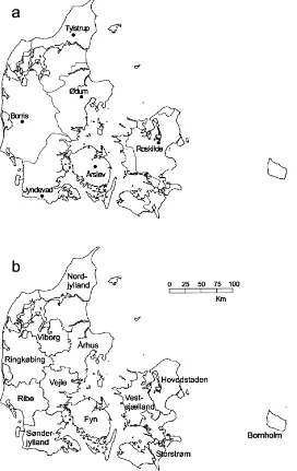
Fig. 1. Regions allocated to six climate stations (a) and administrative counties (b) in Denmark.
temporal variability than the other climatic variables (Table 2). A separate analysis of three different scales of precipitation data was therefore performed.
Six Danish meteorological stations were selected for the upscaling study (Fig. 1a). Climatological nor-mals for the stations are shown in Table 2. Data from the period 1970 to 1997 were used. Missing data for some of the stations were replaced by data from
Table 2
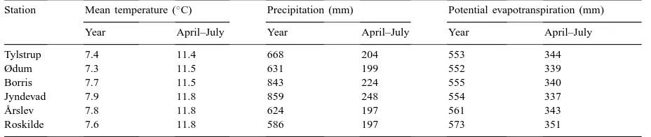
Climatological normals for the six climate stations for the period 1961–1990 (Olesen, 1991) Station Mean temperature (◦
C) Precipitation (mm) Potential evapotranspiration (mm)
Year April–July Year April–July Year April–July
Tylstrup 7.4 11.4 668 204 553 344
Ødum 7.3 11.5 631 199 552 339
Borris 7.7 11.5 843 224 555 340
Jyndevad 7.9 11.8 859 248 554 337
Årslev 7.8 11.8 624 197 561 343
Roskilde 7.6 11.8 586 197 573 351
Each of the six stations was assumed to represent the climate of a region, which was delineated based on a maximum correlation scheme using summer pre-cipitation as the determinant (Fig. 1a). The pairwise correlation of inter-annual variations in total summer precipitation (April–July) between each of the six sta-tions and each of the 650 Danish precipitation stasta-tions was calculated. Only pairs of stations with more than 30 years of data in common for the period 1900–1995 were used. The correlation decreased with increasing distance between the station pairs. For each of the six reference stations a geographical response surface of correlation in summer precipitation was generated us-ing inverse distance interpolation. A composite map was generated by allocating each point (1 km reso-lution) to the reference station with which it has the highest correlation.
Three different spatial scales of precipitation data were used. In the first case precipitation data were taken directly from the climate station that gave the main climatic variables (one or six stations). In the second case the precipitation data from the station pro-viding the climate variables were scaled with the map of relative normal rainfall within 1×1 km2grid cells. This grid map was obtained by interpolation of nor-mal summer rainfall from all 650 Danish precipitation stations relative to each of the six climate stations. In the third case precipitation data were obtained from all 650 precipitation stations with daily data interpolated (inverse distance weighted) onto a 10×10 km2grid. This spatial interpolation may increase the frequency of wet days. An initial test, however, showed that this had no effect of weather on crop yield.
Monthly mean temperatures and precipitation sums were obtained from each year and each county by averaging overall available temperature and station
data within each region. These data were used for estimating effect of temperature and precipitation on measured and simulated yield.
2.3. Soil data
The soil data were composed of two data sets: sur-face soil and subsoil. The sursur-face soil map was based on topsoil texture collected from approximately 32 000 sites on agricultural land at a depth of 0–20 cm (Land-brugsministeriet, 1976). The survey was transformed into a 1:50 000 digital soil data map with eight texture classes (Table 3).
The map of the subsoil defined two types of sub-soil at 1 m depth on arable land in Denmark. The two types were clayey subsoil (more than 10% clay, gener-ally more than 15% clay) and sandy subsoil (less than 10% clay, generally less than 5% clay). The subsoil polygons have been digitised from different geological and soil maps at scales from 1:100 000 to 1:750 000 (Larsen and Sørensen, 1996).
The winter wheat crop was assigned different ef-fective root depths depending on topsoil and subsoil type, resulting in different plant-available water ca-pacities on the different soil types (Table 3). These water capacities were derived from inventories of soil water retention in Danish soils (Madsen and Holst, 1987) and experience on root growth on different soil types (Madsen, 1983; Andersen, 1986).
Table 3
Classification of soil types on agricultural area in Denmark according to surface texturea
Soil type Clay Silt Fine sand Organic matter Area (1000 ha) W (mm)
Sandy Clayey Sandy Clayey
1 0–50 0–200 0–500 <100 761 55 61 85
2 0–50 0–200 500–1000 <100 325 16 120 156
3 50–100 0–250 <100 523 441 105 153
4 100–150 0–300 <100 81 763 145 179
5 150–250 0–350 <100 26 195 156 210
6 250–1000 0–500 <100 20 8 170 227
0–500 200–1000 <100
7 >100 206 31 105 150
8 Atypical 8
Total classified area 1942 1519
aThe characteristics of the soil types are shown in terms of clay (<2
mm), silt (2–20mm), fine sand (20–200mm) and organic matter contents (g kg−1). The area and the capacity for plant available water in winter wheat (W) are shown for each soil type with either a sandy
or a clayey subsoil. The soil type classification does not conform directly with the FAO classification, however, soil types 1 and 2 are mainly sand, type 3 is mainly loamy sand, types 4 and 5 are mainly sandy loam, and type 6 is dominated by loam or sandy clay loam.
2.4. Wheat area
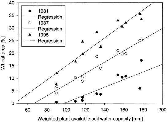
Data on the agricultural area and on the area cropped with winter wheat were obtained from the Danish Bu-reau of Statistics at the county level for every year in the period 1971–1997. The fraction of total agricul-tural area grown with wheat, P (%), in the counties was found in any given year to be a linear function
Fig. 2. Winter wheat area in percent of agricultural area as a function of weighted capacity for plant available water for the soils in the county for three different years. The lines show regression lines for each year separately.
of the area weighted plant-available water capacity of the soil, W (mm):
P = −ab+bW (1)
where a is the soil water capacity at which the area becomes zero (mm), and b is the slope of the regres-sion line (% mm−1). The relationship is illustrated in
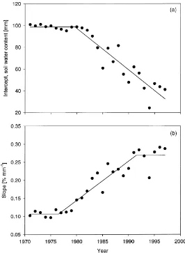
Fig. 3. Intercept (a) and slope (b) of the regression lines relating winter wheat area to capacity for plant available water in the counties in Denmark shown as a function of year. The points represent results from regressions on data from individual years, and the lines show the fitted segmented linear models.
wheat in Denmark increased from 86 500 ha in 1971 to 671 600 ha in 1997. Fig. 2 illustrates that both the slope and the intercept of the regression line relating wheat area to soil water content in the counties changed over this period. This development in the structure of the wheat-growing area is illustrated in Fig. 3 by showing the development of the a and b parameters of Eq. (1) over time. These parameters were estimated by lin-ear regression. Two different segmented linlin-ear models were estimated describing the development of a and
b over time:
a=
a1, y ≤yal
a1+a2(y−yal), yal< y (2)
b=
b1, y ≤ybl
b1+(b2−b1)
y−ybl
ybh−ybl
, ybl< y ≤ybh
b2, ybh< y
(3)
The parameters of Eqs. (2) and (3) were estimated using the NLIN procedure of SAS (SAS Institute, 1996). The parameters of model (2) were estimated as
a1=99 (S.E. 2.6),a2= −3.8 (S.E. 0.36) andyal =
79.6 (S.E. 1.2). The parameters of model (3) were estimated as b1 = 0.107 (S.E. 0.009), b2 = 0.209
(S.E. 0.009), ybl = 76.5 (S.E. 1.4) andybh = 91.5
Two different methods of distributing wheat area within each county were tested, as the actual distri-bution is not known. The first method used a uniform distribution of wheat area across all soil types. The second method used the distribution across soil types implied by Eq. (1), but in such a way that the total wheat area in a county within any given year matched the agricultural statistics. The hypothesis here is that the second method would be superior to the first. Other factors that are correlated with the county structure (e.g., farm types) may, however, also determine which crops are grown, thus making the wheat area less de-pendent on soil type.
2.5. Irrigated area
The agricultural statistics in Denmark provided data at county level on number and size of farms with ir-rigation systems. The proportion of the area of the farms that can be irrigated was taken from an inven-tory published by the Danish Bureau of Statistics in 1976. The irrigated agricultural area in each year and county was then obtained by multiplying the total area of farms with irrigation systems by the proportion of the farm area that can be irrigated. The irrigated area was distributed spatially with preference to soils with low water-holding capacity, W. This was done by let-ting the relative probability of an area being irrigated decline linearly from 1 for soils with W ≤ 60 mm to 0 for soils with W ≥ 160 mm. This function is based on simulated yield effects from using irrigation (Gregersen and Olesen, 1983).
Both the wheat area and the irrigated area were dis-tributed randomly for each year onto a 400×400 m2 grid overlaying the soil maps. Each soil type was as-signed a probability of being irrigated or cropped with wheat based on soil type and method of distribution. This probability depended on the soil water-holding capacity. Grids of different size were tested down to a resolution of 100×100 m2. The results of using the 400×400 m2grid did not deviate from those of a finer spatial resolution. This grid size was therefore cho-sen, because it reduced the number of computations needed.
2.6. Aggregation
The crop model was in each case run for all years for all combinations of soil types, with and without
irrigation, within each of the climatic regions and/or grid boxes. The aggregated county or national yields (Mg ha−1) were calculated as the area weighted sums
of these simulated yields.
2.7. Evaluation
The relationship between observed and simulated county yields were first analysed using the following statistical model, which takes the observed yields to be a function of systematic effects (year and simulated yields) and random effects (county and residual):
Yyc=α+βy+δXyc+Gc+Eyc (4)
where Yyc is the observed yield in county c in year
y, and Xyc is simulated yield.α, β, and δ are fixed effects. G and E are random effects associated with county and the county/year combination, respectively. This model was analysed for each spatial combination using the MIXED procedure of SAS (SAS Institute, 1996).
Subsequently the observed and simulated county and national yields were detrended to a 1990 basis using separate linear time trends for each county estimated by linear regression. The ability of the model and the upscaling method to capture the inter-annual variability in yields was evaluated for county and national levels by linear regression of observed detrended yield on simulated detrended yield. At county level this measure includes the ef-fect of systematic differences between counties. In addition a linear regression of observed on simulated county residuals from the linear technology trend was performed.
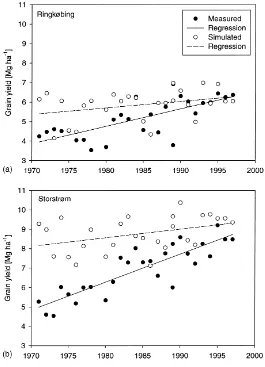
Fig. 4. Time trend of observed (d) and simulated (s) grain yield for winter wheat for two counties (Ringkøbing and Storstrøm). The simulated yields were calculated using scale 6GP with a uniform distribution of winter wheat area within each county.
3. Results
There were large differences in observed and simulated responses between the counties as illus-trated in Fig. 4. The observed yield trend for win-ter wheat was much steeper for Storstrøm county (0.15 Mg ha−1yr−1) than for Ringkøbing county
(0.10 Mg ha−1yr−1). The yield level was highest in
Storstrøm county, giving an annual yield increase of 2.0% in Storstrøm county and 1.7% in Ringkøbing county. Storstrøm county is dominated by loamy soils, whereas Ringkøbing county is dominated by sandy soils. The simulated yield trends showed tendencies
of increasing yields, but these were in most cases not significant.
The effect of the different scales of soil and climate data on mean and standard deviation of simulated na-tional grain yield and irrigation demand is shown in Table 4. Mean simulated, detrended yield was about 1 Mg ha−1higher than the observed for an even wheat
area distribution and about 1.5 Mg ha−1 higher than
Table 4
Measured and simulated national winter wheat grain yield and irrigation amounts for different scales of climate and soil data and two different methods of distributing wheat area within each countya
Scale of input data Uniform distribution Soil type-dependent distribution Mean yield
Measured 6.57 0.62 6.57 0.62
1OP 7.61 0.89 20.3 8.39 0.90 10.4
1RP 7.61 0.90 20.2 8.38 0.90 10.7
1GP 7.35 0.88 20.0 8.11 0.94 11.6
6OP 7.51 0.77 20.5 8.25 0.77 11.7
6RP 7.59 0.76 19.9 8.31 0.77 10.9
6GP 7.61 0.77 20.5 8.34 0.78 11.3
1OG 7.54 0.88 16.4 7.91 0.88 10.2
1OC 7.44 0.90 15.3 7.38 0.90 10.3
1RG 7.54 0.89 16.3 7.91 0.89 10.4
1RC 7.44 0.91 15.5 7.38 0.91 10.6
aThe notation for scale of input data is explained in Table 1. Both observed and simulated yields were detrended and adjusted to 1990
level using a linear technology trend.
considerably decreased mean simulated grain yield and irrigation demand. Simulated irrigation demand decreased by 25–50% when changing from the uni-form to the soil type-dependent distribution of the wheat area.
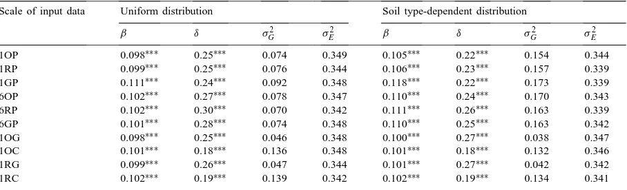
Table 5 shows the analysis of county yields using the statistical model in Eq. (4). The slopes of the re-sponse of observed to simulated yields were in the range 0.18–0.30. The values increased slightly when using six versus only one climate station, and were lowest at the coarsest resolution of soil data. The two
Table 5
Analysis of the relation between observed and simulated county yields using the statistical model in Eq. (4) for different scales of climate and soil data and two different methods of distributing wheat area within each countya
Scale of input data Uniform distribution Soil type-dependent distribution
β δ σ2
aThe notation for scale of input data is explained in Table 1.βandδare the slopes of effects of year and simulated yields, respectively.
σ2
G andσE2 are the error variances associated with counties and residuals, respectively. ∗p<0.05;∗∗p<0.01;∗∗∗p<0.001.
Table 6
Coefficient of determination (R2) for linear regression of simulated on measured Danish county and national yields from 1971 to 1997 for
different scales of climate and soil data and two different methods of distributing wheat area within each countya
Scale of input data Uniform distribution Soil type-dependent distribution
National yield County yield County residuals National yield County yield County residuals
1OP 0.12 0.36∗∗∗ 0.08∗∗∗ 0.14 0.31∗∗∗ 0.08∗∗∗
1RP 0.13 0.37∗∗∗ 0.09∗∗∗ 0.15∗ 0.31∗∗∗ 0.09∗∗∗
1GP 0.14 0.39∗∗∗ 0.08∗∗∗ 0.16∗ 0.32∗∗∗ 0.09∗∗∗
6OP 0.13 0.36∗∗∗ 0.09∗∗∗ 0.14 0.30∗∗∗ 0.08∗∗∗
6RP 0.15∗ 0.37∗∗∗ 0.10∗∗∗ 0.16∗ 0.31∗∗∗ 0.09∗∗∗
6GP 0.13 0.36∗∗∗
0.08∗∗∗
0.15∗
0.31∗∗∗
0.09∗∗∗
1OG 0.12 0.38∗∗∗
0.08∗∗∗
0.13 0.39∗∗∗
0.09∗∗∗
1OC 0.12 0.25∗∗∗
0.08∗∗∗
0.12 0.25∗∗∗
0.08∗∗∗
1RG 0.13 0.39∗∗∗
0.09∗∗∗
0.14 0.40∗∗∗
0.10∗∗∗
1RC 0.13 0.25∗∗∗
0.09∗∗∗
0.13 0.26∗∗∗
0.10∗∗∗
aThe notation for scale of input data is explained in Table 1. The significance level is based on an F-test of the slope in the regression.
Both observed and simulated yields were detrended and adjusted to 1990 level using a linear technology trend. The linear regression was performed for detrended national yields, detrended county yields and for residuals obtained from linear regression of yields on year for each county.
∗p<0.05;∗∗p<0.01;∗∗∗p<0.001.
The effect of using different scales of climate and soil data on the ability of the model to explain inter-annual variability in yield is shown in Table 6. The coefficients of determination for both national yield and for county residuals were low and largely unaffected by scale of climate or soil data.
The coefficient of determination was higher for county compared with national detrended yields
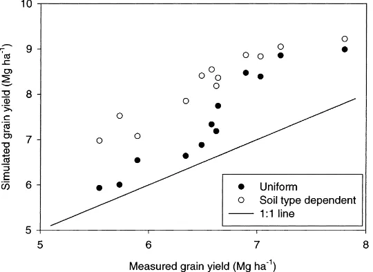
Fig. 5. Simulated mean grain yield versus measured mean grain yield scaled to 1990 level for each county. The simulated yields were calculated using scale 6GP for either a uniform distribution of wheat area or a soil type-dependent distribution of wheat area within each county.
(Table 6). This reflects the fact that simulated and measured mean wheat yields varied between counties (Fig. 5). There was a slightly more linear relation-ship between simulated and measured yield for the uniform distribution of wheat area.
Fig. 6. Coefficient of determination (R2) of linear regressions of simulated on measured detrended Danish county yields for each county
plotted versus weighted soil water holding capacity of the county for two scales; 1OP and 6GP. The wheat area was distributed evenly on all soil types within each county. The lines show the linear regressions of R2 on soil water-holding capacity.
Table 7
Regression of simulated correlation on observed correlation bet-ween detrended yields in different counties for different scales of climate and soil data and two different methods of distributing wheat areaa
aThe notation for scale of input data is explained in Table 1.
Both the slope and coefficient of determination (R2) of the
regres-sions are shown. ∗
p<0.05;∗∗
p<0.01;∗∗∗ p<0.001.
coefficients of determination were obtained for coun-ties with high soil water capacicoun-ties. This was espe-cially the case when six climate stations were used for the upscaling.
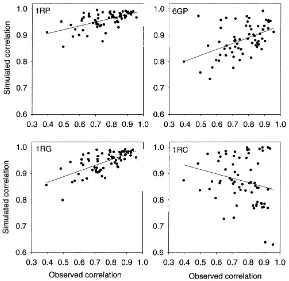
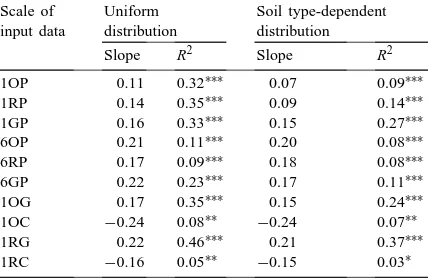
The simulated spatial autocorrelation was in most cases much higher than the observed autocorrelation (Fig. 7). Increasing the number of climate stations from one to six or using the much larger network of precipitation stations reduced the simulated autocorre-lations. This was reflected in the slope of the line relat-ing simulated to observed spatial correlation (Table 7), but not necessarily in the coefficient of determination of that relationship. The use of dominant soil types on the county scale also reduced the simulation correla-tion, but the slope of the relationship was reversed.
Table 8 shows the slopes of linear regressions of simulated and observed detrended county yields on
Table 8
Slope of regression of simulated or measured detrended yield on temperature or precipitation for the periods April–July and October–July Precipitation, April–July (mm) −0.004∗∗∗
−0.001 Precipitation, October–July (mm) −0.002∗∗∗
−0.003∗∗∗ ∗p<0.05;∗∗p<0.01;∗∗∗p<0.001.
temperature and precipitation for either the whole growing season (October–July) or the main growing season (April–July). The signs of the response of both simulated and observed yield to temperature and precipitation were identical, but the significance of the response was higher for observed yields.
4. Discussion
The scales of soil and climate data applied here had only a small effect on the ability of the model to repro-duce the inter-annual variability in county and national yields (Table 6). The ability of the model to reproduce the observed spatial variation in yields was, however, substantially reduced when the resolution of soil data was reduced to county level, which can be seen from the increase in the random error associated with coun-ties (Table 5). Decreasing the resolution of soil data to both the 10×10 km2grid net and to county level sub-stantially reduced mean national simulated yields, es-pecially when the soil type dependent distribution was used (Table 4). Decreasing the spatial resolution of soil data to a county level completely destroyed the abil-ity of the simulated results to represent the observed spatial autocorrelation structure (Fig. 7 and Table 7). All these effects were brought about by changes in the weight with which different soil types contributed to regional and national yields. This also had large effects on simulated irrigation demand (Table 4). The results thus collectively suggest that the spatial resolution of soil data should be 10×10 km2or finer.
management). The results also show that a relatively high spatial resolution of climate data is necessary to represent the observed spatial autocorrelation.
Easterling et al. (1998) used a simulation model to estimate wheat and maize yields in the central Great Plains of USA. They found that disaggregating climate and soil data to approximately 1◦×1◦
resolu-tion gave the best agreement between simulated and observed yields. Denmark spans 3◦ of latitude and
7◦ of longitude. A resolution of 1◦×1◦ is
compara-ble to the use of six climate stations and soil data from a 10×10 km2 grid applied here. This rather detailed level of climate data was, however, only of some advantage for description of the inter-annual yield variation at county level, whereas the ability to describe variation in national yields was largely unaffected by scale of climate data.
The proportion of the inter-annual variation in ob-served yields captured by the model was substantially higher in counties with higher water-holding capaci-ties (Fig. 6). There are two possible reasons for this. Firstly, yields are generally lower on sandy soils and crops here tend not only to suffer from lack of wa-ter, but also from a higher risk of nutrient deficiency and from a higher disease prevalence such as take-all (Bødker et al., 1990). Secondly, the proportion of livestock farms is much higher in counties with sandy soils. The livestock density of cattle and pigs in 1997 was 0.3–0.5 LU ha−1in counties dominated by loamy
soils and 0.9–1.1 LU ha–1 in counties dominated by sandy soils. Dairy farmers in Denmark often use win-ter wheat as a break crop in their forage crop rotation, and less emphasis is therefore put on optimal manage-ment of the crop. Similar effects have been observed for cereals used as break crops in vine rotations in Southern France (Wassenaar et al., 1999) and for soybean (Glycine max [L.] Merr.) yields in areas of cattle production in Iowa, USA (Haskett et al., 1995). The result of these effects is that, as the spatial extent of the model is increased, it gradually subsumes more elements of the landscape and the ecosystem that are not formally included in the model (Rastetter et al., 1992). This results in reduced ability of the model to properly simulate inter-annual variability in crop yields at the aggregate level.
Even though the model only explained a very small proportion of the observed inter-annual yield variabil-ity, the response of the simulated yields to seasonal
average temperature variability matched that of the observed yields (Table 8). This was to some extent also the case for effects of seasonal rainfall on yield. There was no significant trend in any of these climate variables. The effects in Table 8 are therefore caused by the inter-annual variability in climate, and the de-trending of both simulated and observed yields mainly corrects for technological and land-use effects.
The results in Table 8 are in line with results reported by Easterling et al. (1996), who used a sim-ulation model run for representative farms in seven counties to calculate crop production in eastern Ne-braska. The model was found to reliably estimate crop yields under temperature extremes, whereas the model failed to simulate effects on yield of extremes in rain-fall. The crop models thus capture some of the broad effects of climate, especially those of temperature.
The use of different distributions of wheat area across the different soil types had no substantial ef-fects on the ability of the model to mimic inter-annual yield variations (Tables 5 and 6). It, however, resulted in a change in the relationship of observed to simulated mean county yields (Fig. 5). The soil type-dependent distribution resulted in considerably higher simulated yields, especially on the sandier soils. Assuming that the simulated mean county yields should be propor-tional to the observed yields, then desired simulated values should be somewhere between those simulated by the two different methods of distributing wheat area. This indicates that wheat area is not uniformly distributed on all soil types within a county. However, the relationship between wheat area and soil water ca-pacity estimated from the county data may not strictly apply within counties.
5. Conclusions
For the estimation of aggregated effects of climate change on national productivity of winter wheat it is not necessary to apply spatially detailed climate infor-mation for Denmark. Climate data from one centrally placed station will be sufficient. An increased spatial resolution of climate data will, however, be necessary if the productivity of regions or counties are to be considered.
information on the spatial aspects of yield variability. Different processes became dominant depending on which measures were evaluated and at which scale. Studies on the upscaling of indicators of agricultural productivity should therefore consider indicators of temporal, spatial and the interaction of temporal and spatial variation. In the current study, these effects were simulated through the interaction between soils and climate, but other factors may also be important for upscaling indicators of agricultural production. Such geographically variable factors might include farm structure, management, landscape, and agricul-tural and environmental policies.
The ability of the upscaling method to predict both the regional and inter-annual variation in yields may be improved through better methods of distributing the wheat area across soil types. This could be obtained by setting up a number of representative farm types and relate the wheat area to farm types and the farm types to soil types. This would also allow for the effect of farm type on yield to be incorporated explicitly in the upscaling procedure.
Acknowledgements
The work was supported by the European Union under contract ENV4-CT95-0154.
References
Andersen, A., 1986. Rodvækst i forskellige jordtyper. Tidsskr. Planteavls Specialserie S1827. Lyngby, Denmark.
Aslyng, H.C., Hansen, S., 1982. Water balance and crop production simulation. The Royal Veterinary and Agricultural University, Copenhagen.
Asseng, S., van Keulen, H., Stol, W., 2000. Performance and application of the APSIM Nwheat model in the Netherlands. Eur. J. Agron. 12, 37–54.
Bødker, L., Schulz, H., Kristensen, K., 1990. Influence of cultural practices on incidence of take-all (Gaemannomyces graminis var tritici) in winter wheat and winter rye. Tidsskr. Planteavl. 94, 201–209.
Brown, R.A., Rosenberg, N.J., 1997. Sensitivity of crop yield and water use to change in a range of climatic factors and CO2
concentrations: a simulation study applying EPIC to the central USA. Agric. Forest Meteorol. 83, 171–203.
Davies, A., Jenkins, T., Pike, A., Shao, J., Carson, I., Pollock, C.J., Parry, M.L., 1997. Modelling the predicted geographic and economic response of UK cropping systems to climate change scenarios: the case of potatoes. Ann. Appl. Biol. 130, 167–178.
Dhakhwa, G.B., Campbell, C.L., LeDuc, S.K., Cooter, E.J., 1997. Maize growth: assessing the effects of global warming and CO2 fertilization with crop models. Agric. For. Meteorol. 87,
253–272.
Easterling, W.E., Chen, X., Hays, C.J., Brandle, J.R., Zhang, H., 1996. Improving the validation of model-simulated crop yield response to climate change: an application of the EPIC model. Clim. Res. 6, 263–273.
Easterling, W.E., Weiss, A., Hays, C.J., Mearns, L.O., 1998. Spatial scales of climate information for simulating wheat and maize productivity: the case of the US Great Plains. Agric. For. Meteorol. 90, 51–63.
Gregersen, A.K., Olesen, J.E., 1983. Sandsynlige merudbytter ved vanding i vårbyg, græs og kartofler. Tidsskr. Planteavls Specialserie S1668. Lyngby, Denmark.
Grindlay, D.J.C., 1997. Towards an explanation of crop nitrogen demand based on the optimization of leaf nitrogen per unit leaf area. J. Agric. Sci., Camb. 128, 377–396.
Harrison, P.A., Butterfield, R.E., 1996. Effects of climate change on Europe-wide winter wheat and sunflower productivity. Clim. Res. 7, 225–241.
Haskett, J.D., Pachepsky, Y.A., Acock, B., 1995. Estimation of soybean yields at the county and state levels using GLYSIM: a case study for Iowa. Agron. J. 87, 926–931.
Jamieson, P.D., Semenov, M.A., Brooking, I.R., Francis, G.S., 1998. Sirius: a mechanistic model of wheat response to environmental variation. Eur. J. Agron. 8, 161–179.
Jamieson, P.D., Porter, J.R., Semenov, M.A., Brooks, R.J., Ewert, F., Ritchie, J.T., 1999. Comments on “Testing winter wheat simulation models predictions against UK grain yields” by Landau et al. (1998). Agric. For. Meteorol. 96, 157–161. Knudsen, L., Birkmose, T., Østergaard, H.S., 1997. Gødskning
og kalkning. In: Pedersen, C.Å. (Ed.), Oversigt over Lands-forsøgene. Landbrugets Rådgivningscenter, Skejby, Denmark, pp. 150–194.
Landau, S., Mitchell, R.A.C., Barnett, V., Colls, J.J., Craigon, J., Moore, K.L., Payne, R.W., 1998. Testing winter wheat simu-lation models’ predictions against observed UK grain yields. Agric. For. Meteorol. 89, 85–99.
Landbrugsministeriet, 1976. Den danske jordklassificering. Teknisk redegørelse. Ministry of Agriculture, Copenhagen.
Larsen, P., Sørensen, M.B., 1996. Geographic data at the Depart-ment of Landuse. SP Report No. 6. Research Centre Foulum, Denmark.
LeDuc, D.K., Holt, D.A., 1987. The scale problem: modeling plant yield over time and space. In: Wisiol, K., Hesketh, J.D. (Eds.), Plant Growth Modeling for Resource Management, Vol 1. CRC Press, Boca Raton, pp. 125–137.
Madsen, H.B., 1983. Himmerlands Jordbundsforhold. C.A. Reitzels Forlag, Copenhagen.
Madsen, H.B., Holst, K., 1987. Potentielle marginaljorder. Mar-ginaljorder og miljøinteresser. Miljøministeriets projektundersø-gelser. Teknikerrapport No. 1. Ministry of Environment, Copenhagen.
Olesen, J.E., 1991. Agrometeorological Annual Report 1990. Tidsskr. Planteavls Specialserie S2130. Lyngby, Denmark. Olesen, J.E., Plauborg, F., 1995. MVTOOL Version 1.10 for
developing MARKVAND. SP Report No. 27. Research Centre Foulum, Denmark.
Olesen, J.E., Jensen, T., Petersen, J., 2000. Sensitivity of field-scale winter wheat production in Denmark to climate variability and climate change. Clim. Res., in press.
Orson, J.H., 1995. Crop protection practices in wheat and barley crops. In: Hewitt, H.G., Tyson, D., Holloman, D.W., Smith, J.M., Davies, W.P., Dixon, K.R. (Eds.), A Vital Role for Fungicides in Cereal Production. BIOS Scientific Publishers, Cirencester, UK, pp. 9–18.
Plantedirektoratet, 1997. Vejledning og skemaer, mark og gødningsplan, gødningsregnskab, grønne marker 1997/1998. Plantedirektoratet. Lyngby, Denmark.
Plauborg, F., Andersen, M.N., Heidmann, T., Olesen, J.E., 1996. MARKVAND: an irrigation scheduling system for use under limited irrigation capacity in a temperate humid climate. In: Smith, M., Pereira, L.S., Berengena, J., Itier, B., Goussard, J., Ragab, R., Tollefson, L., van Hofwegen, P. (Eds.), Irrigation Scheduling: From Theory to Practice. FAO, Rome, pp. 177–184.
Rastetter, E.B., King, A.W., Cosby, B.J., Hornberger, G.M., O’Neill, R.V., Hobbie, J.E., 1992. Aggregating fine-scale ecological knowledge to model coarser-scale attributes of ecosystems. Ecol. Appl. 2, 55–70.
Rietveld, M.R., 1978. A new method for estimating the regression coefficients in the formula relating solar radiation to sunshine. Agric. Meteorol. 19, 243–252.
SAS Institute, 1996. SAS/STAT software: changes and enhancements through release 6.11. Cary, NC.
Semenov, M.A., Wolf, J., Evans, L.G., Eckersten, H., Iglesias, A., Porter, J.R., 1996. Comparison of wheat simulation models under climate change. II. Application of climate change scenarios. Clim. Res. 7, 271–281.
Silvey, V., 1994. Plant breeding in improving crop yield and quality in recent decades. Acta Hort. 355, 19–34.
Sylvester-Bradley, R., Scott, R.K., Stokes, D.T., Clare, R.W., 1997. The significance of crop canopies for N-nutrition. Aspects Appl. Biol. 50, 103–116.
van Keulen, H., Stol, W., 1991. Quantitative aspects of nitrogen nutrition in crops. Fert. Res. 27, 151–160.