isprs annals III 3 11 2016

INVARIANT DESCRIPTOR LEARNING USING A SIAMESE CONVOLUTIONAL

NEURAL NETWORK

L. Chen*, F. Rottensteiner, C. Heipke

Institute of Photogrammetry and GeoInformation, Leibniz Universität Hannover, Germany - (chen, rottensteiner, heipke)@ipi.uni-hannover.de

Commission III, WG III/1

KEY WORDS: Descriptor Learning, CNN, Siamese Architecture, Nesterov's Gradient Descent, Patch Comparison

ABSTRACT:

In this paper we describe learning of a descriptor based on the Siamese Convolutional Neural Network (CNN) architecture and evaluate our results on a standard patch comparison dataset. The descriptor learning architecture is composed of an input module, a Siamese CNN descriptor module and a cost computation module that is based on the L2 Norm. The cost function we use pulls the descriptors of matching patches close to each other in feature space while pushing the descriptors for non-matching pairs away from each other. Compared to related work, we optimize the training parameters by combining a moving average strategy for gradients and Nesterov's Accelerated Gradient. Experiments show that our learned descriptor reaches a good performance and achieves state-of-art results in terms of the false positive rate at a 95% recall rate on standard benchmark datasets.

* Corresponding author

1. INTRODUCTION

Feature based matching for finding pairs of homologous points in two different images is a fundamental problem in computer vision and photogrammetry, required for different tasks such as automatic relative orientation, image mosaicking and image retrieval. In general, for a feature based matching algorithm one needs to define a feature detector, a feature descriptor and a matching strategy. Each of these three modules is relatively independent of the others, therefore a combination of different detectors, descriptors and matching strategies is always possible and a good combination might adapt to some specific data configurations or applications. The key problem of image matching is to achieve invariance against possible photometric and geometric transformations between images. The list of photometric transformations that affects the matching performance comprises illumination change, different reflections and the use of different spectral bands in the two images. Geometric transformations comprise translation, rotation and scaling as well as affine and perspective transformation; besides, the matching performance may also be affected by occlusion caused by a viewpoint change. In most cases, features for matching are extracted locally in the image, and a feature vector (descriptor) used to represent the local image structure is generated from a relatively small local image patch centred at each feature. Consequently, it is usually suf-ficient to design a matching strategy that is invariant to affine distortion, because a global perspective transformation can be approximated well by an affine transformation locally. Such distortions are likely to occur in case of large changes of the view points and the viewing directions.

Classical descriptors, like SIFT (Lowe, 2004) and SURF (Bay et al., 2008) are designed manually; they are invariant to shift, scale and rotation, but not to affine distortions. Some authors (Mikolajczyk and Schmid, 2005; Moreels and Perona, 2007; Aanæs et al., 2012) have evaluated the performance of detectors

and descriptors against different types of transformations in planar and 3D scenes, using recall and matching precision as the main evaluation criteria (Mikolajczyk and Schmid, 2005). As discussed in (Moreels and Perona, 2007), their results show that the performance of classical detectors and descriptors drops sharply when the viewpoint change becomes large, because the local patches vary severely in appearance, so that the tolerance of classical feature detectors and descriptors is exceeded.

One strategy to improve the invariance of descriptors to view point changes is to convert the descriptor design and descriptor matching into a pattern classification problem. By collecting the patches of the same feature in different images, one can capture the real differences between these patches. The process of designing invariant feature descriptors is equal to finding a mapping of those patches into a proper feature space where they are located more closely to the descriptors of the homologous features. By using an appropriate machine learning model, a loss based on the similarity of the learned descriptors is designed. In this case, decreasing the loss by learning helps to achieve a higher level of invariance.

In this paper, we present a new method for defining descriptors based on machine learning. It extends our previous descriptor learning work on Convolutional Neural Networks (CNN; Chen et al., 2015). As a CNN has a natural "deep" architecture, we expect this architecture to have a stronger modelling ability which can be used to produce invariance against more challenging transformations, which classical manually designed descriptors cannot cope with. By conducting the training in a mini-batch manner, using a moving average strategy on gradients and a momentum term as well as Nesterov's Accelerated Gradient, we optimize the training parameters and achieve our trained descriptor. The main contribution of this paper is that we first introduce this training algorithm into descriptor learning tasks based on Siamese CNN.

2. RELATED WORK

A substantial body of classical descriptors are designed in a manual manner, for instance SIFT (Lowe, 2004) or SURF (Bay et al., 2008). More recent manually designed methods like DAISY (Tola et al., 2010) introduced a more complex pattern of pooling operations. These descriptors have been considered to be a standard for quite some time. However, they cannot deal with large viewpoint changes. This is why affine-invariant frameworks for feature based matching have been proposed, e.g. ASIFT (Morel and Yu, 2009). By using an affine view-sphere simulation strategy, ASIFT transforms the two original images to many affine versions, then features and descriptors are computed based on those images. Afterwards the descriptors from affine distorted versions of the two original images are matched. As each feature has many different descriptors that are built on simulated affine views, ASIFT can cope with affine distortions better than other matching algorithms that only run on original images. However, ASIFT is computationally expensive and benefits from the view-sphere simulation matching scheme rather than from any improvements on viewpoint invariance of the feature descriptor.

An alternative to using hand-crafted features and strategies such as sampling many potential viewpoints synthetically is descriptor learning (Bengio et al., 2013). To test if machine learning approaches can achieve better results, Brown et al. (2011) proposed a descriptor learning framework, in which a descriptor is composed of four different modules: 1) Gaussian smoothing; 2) non-linear transformation; 3) spatial pooling or embedding; 4) normalization. New descriptors can be derived by optimizing the configuration of the second and the third modules. An extension of their work which allows convex optimization in the training process is given in (Simonyan et al., 2012; 2014). In (Trzcinski et al., 2012; 2015), a descriptor learning architecture based on the combination of weak learners by boosting is designed, in which the weak learners rely on comparisons of simple features. In the training process, the optimal features for the weak learners are determined along with the optimal matching score function. The resulting descriptor outperforms SIFT under nearly every type of transformation on the benchmark data set of Mikolajczyk and Schmid (2005).

Another category of descriptor learning frameworks is built on CNN. CNN consists of multiple convolutional layers (LeCun et al. 1998). Invariant feature representation learning based on a so-called Siamese CNN has originally been proposed in (Bromley et al., 1993) to extract feature representations for signature verification, where the signatures from one person may change in complex ways, which are nearly impossible to capture with explicit models. The term Siamese refers to the fact that the same CNN architecture and the same parameters are applied to two input data sets with complex relative distortions. In (Hadsell et al., 2006), the Siamese CNN architecture was used to learn feature representations for digit recognition; as the same digit written by different people varies considerably, a Siamese CNN architecture is used to find an invariant feature representation that can map the high dimensional input data into a more discriminative feature space where "similar" digits are located more closely to each other. This feature space is defined by the output of the final convonlutional layer of the CNN. The use of multiple layers (i.e., the deep architecture) is the reason for the strong modelling ability of CNNs. This property fits well with the requirements for learning descriptors that are invariant against various types of transformations. Consequently, CNN have been used to train descriptors for patch comparison.

The first patch comparison work based on the Siamese CNN was presented in (Jahrer et al., 2008). Jahrer et al. (2008) used the Siamese CNN to train the descriptor and compare the patches, but the training data was generated from image warps and dependent on input images, which makes this method less practical, because it always needs a prior simulation and training before image matching. In (Osendorfer et al., 2013), a Siamese CNN is used to train a descriptor; the paper focuses on the comparison of four different types of loss functions. More recently, the Siamese architecture was used to train patch descriptors to cope with dynamic lighting conditions (Carlevaris-Bianco and Eustice, 2014), feeding patches with severe illumination change into a Siamese CNN; illumination invariance that exceeds any hand-crafted descriptors is achieved. In (Lin et al., 2015), images taken from aerial and terrestrial views are fed into a Siamese CNN network, followed by applying a similarity function that indicates whether the two images contain identical scenes. Using this model, aerial and terrestrial view are linked, which can be used to generate a relation graph. However, the descriptor is applied to the whole image, not to patches centred around feature points, therefore it can only build rough connections on the level of complete images, and it cannot find precise point correspondence.

Our work is closely linked to the work in (Han et al., 2015; Zagoruyko and Komodakis, 2015; Zbontar and Lecun, 2015). Han et al. (2015) and Zagoruyko and Komodakis (2015) did not only train the descriptor, but also a classifier to determine the matching label, which is called the metric network (Han et al., 2015) and decision layer (Zagoruyko and Komodakis, 2015). This makes their model more complicated than ours. Zbontar and LeCun (2015) also calculate four extra layers of the metric network, but apply them to wide baseline dense stereo matching rather than to feature based matching for orientation. They currently achieve the best result on the KITTI benchmark.

If one trained a metric function for pairs of patches, then every pair of feature patches should be fed into the network with metric layers when this descriptor is applied in real image matching or large scale image retrieval. In this case, the highly efficient search strategies such as Best Bin First (Beis and Lowe, 1997) in a KD tree cannot be used and the matching speed is seriously influenced. This reduces the practical value of a learned descriptor in feature based image matching. In contrast to those works, we therefore train a descriptor without a metric function for the two patches.

3. METHODOLOGY

In this section the Siamese descriptor learning architecture is described first. Then, details of the CNN used in this architecture are presented. Finally, we describe the method used to learn the parameters of the CNN.

3.1 Siamese Descriptor Learning: Architecture

In order to learn the CNN-based descriptor, we need pairs of training patches of which we know whether they represent homologous image features or not. In this context, it is important that the set of positive examples (the pairs that correspond to homologous key points) contains transformations that the learned descriptor should be tolerant to. The basic idea of the Siamese architecture for descriptor learning is to apply the same type of CNN using the same set of parameters  to each of the patches that should be checked for correspondence ISPRS Annals of the Photogrammetry, Remote Sensing and Spatial Information Sciences, Volume III-3, 2016

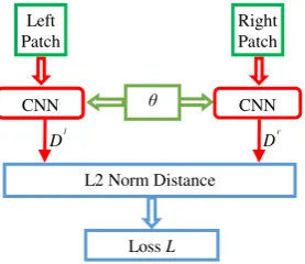
and determine these parameters by optimising a loss function of the L2 norm of the differences of the resultant descriptors. That is, by adjusting the parameters so that the L2 norm is as discriminative as possible in separating correct from incorrect matches we obtain a descriptor that should be tolerant to the type of geometric distortions that occur between positive examples in the training data; refer to Figure 1 for an illustration of the whole architecture. In the following section, the parameters are explained in detail.

Figure 1. The architecture for Siamese CNN descriptor learning used in this paper. Green: input patches; Red: a CNN as depicted in figure 3; Dl, Dr: descriptors for the right and the left image patch, respectively. Blue: loss function. The two CNNs share the learned parameters  (orange).

In the training process, the following loss function based on the L2 norm of the differences of the CNN descriptors of training function creates a margin between matching and non-matching pairs. For matching pairs, a distance larger than a “pull radius” lpull is penalised, whereas for non-matching pairs (the negative training examples), penalisation occurs for distances smaller than a “push radius” lpush. This type of loss function has been shown to be suitable for descriptor learning by Osendorfer et al. (2013). The two radii are parameters that have to be set by the user. The CNN parameters are initialised at random, so that initially the distances of descriptors from matching pairs cannot be expected to be small. The learning procedure then tries to find parameters  of the CNN that push the descriptors of unmatched pairs away from each other in feature space, while

pulling the descriptors of matching pairs closer to each other. An illustration of this idea is shown in Figure 2. Before learning, the descriptors are distributed randomly in feature space, while after learning the descriptors from patches corresponding to homologous points lie close to each other.

Figure 2. Descriptor learning. In the top part, each coloured dot represents a descriptor; identical colours indicate homologous patches from multi-view images. In the lower part, the radius of the inner concentric circle is lpull and the radius of the outer one is lpush.

3.2 CNN Descriptor

The concept of CNNs was proposed by (LeCun et al. 1998); it is a multi layer neural network. A CNN may have one or several stages consisting of a convolution layer, a nonlinear layer and a feature pooling layer each. Compared to general multi layer neural networks, there are two main differences:

1) In the convolution layer, the neurons of the input layer are not fully connected to those of the next layer and weights are shared, so that the same weights are repeatedly used across the different position of the input layer. This is the reason for using the term "convolutional" network. The weight sharing strategy dramatically decreases the number of parameters and makes deep architectures consisting of larger numbers of stages trainable.

2) The network decreases the layer size in successive stages by pooling layers. Therefore, the input can be compressed into a meaningful feature representation, which reduces the dimension of the original data considerably.

In essence, a CNN can be seen as a nonlinear mapping function, transforming the input (a given image patch) to a higher-level but lower dimensional feature representation.

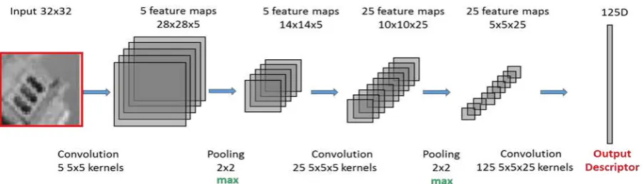
In this paper, we use a CNN architecture consisting of three stages to learn feature descriptors (cf. figure 3). Details about the architecture and the learning parameters are listed in table 1. The input patch size is 32 by 32 pixels. The CNN contains three stages. The first two stages have a [convolution - nonlinear - pooling] structure, whereas the third one only contains a convolution layer. For each stage k with k  {1, 2, 3}, the parameters to be determined are the convolution kernel wk and the bias term bk, which, thus, constitute the parameters  shared by the two CNNs in the Siamese architecture. For brevity, it is also written as parameters wk and bk in the remain text. Whereas in the first convolution layer we train five 2D kernels of size 5 x 5 to produce five feature maps, in the subsequent stages we determine the parameters of 3D kernels (25 5 x 5 x 5 kernels in stage 2; 125 5 x 5 x 25 kernels in stage 3). The nonlinearity is

Figure 3. The CNN used in this paper to learn the descriptor Input Convolution

kernels

Nonlinear Pooling Output Learning parameters

Stage 1 32 x 32 5 x 5 x 5 sigmoid max (2 x 2) 14 x 14 x 5 w1 , b1

Stage 2 14 x 14 x5 25 x 5 x 5 x 5 sigmoid max (2 x 2) 5 x 5 x 25 w2 , b2

Stage 3 5 x 5 x 25 125 x 5 x 5 x 25 ~ ~ 1 x 1 x 125 w3 , b3

Table 1. Detailed architecture and learning parameters for the CNN used in this paper. The numbers indicate pixel numbers.

based on the sigmoid function and we use max pooling (without overlap, i.e. stride = 2), preserving the largest value in a 2 x 2 neighbourhood as the output. The final output of our CNN is a 125 dimensional vector. This 125 dimensional vector is the learned descriptor that is used to represent the content of a local image patch surrounding a feature.

The CNN architecture used in this paper is different from (Han et al., 2015; Zagoruyko and Komodakis, 2015). First, a smaller input window with only 32 x 32 pixels (instead of 64 x 64 pixels, which were used in the reported work), is employed. When processing wide baselines images, the appearance of patches surrounding feature points changes more severely than in narrow baseline situations. By using of smaller context window, the proposed descriptor can potentially cope with larger deformations in a better way. Additionally, the sigmoid function is applied to achieve nonlinearity because we found it to perform better than the Rectified Linear Unit (ReLU). Finally, compared to the related work, we use a more advanced training algorithm (see section 3.3).

3.3 Training of the Siamese CNN

Training of the CNN is based on gradient descent to find the optimum of the loss function. In this context, the well-known back propagation algorithm (Rumelhart et al., 1986) can be used to determine derivatives of the loss with respect to the parameters. In our network, back-propagation is a little more complicated than usual, because the gradients are influenced by both subnets in the Siamese CNN. In Section 3.3.1 the online gradient training procedure is described, whereas Section 3.3.2 contains details about the way in which gradients are computed.

3.3.1 Mini-batch Gradient Descent: In general, after calculating the gradient of the loss function with respect to the parameters to be learned, the parameters are updated according to the gradient, taking into account a learning rate . In the literature one can find methods using all training samples to compute the gradients (batch training) and online methods, using only one training sample at a time (Bishop., 2006). The first variant can be very slow in the presence of many training samples. On the other hand, online gradient descent can be unstable because of sampling errors when computing the

gradient only from one sample. As a compromise we use mini-batch gradient descent, updating the parameters on the basis of gradients computed from relatively small groups of training samples in each iteration. Each group (mini-batch) typically contains hundreds or several thousands of training samples. The gradients used to update the parameters are average gradients over all samples in the group currently considered.

One way of gradient descent is to consider a fixed learning rate

 and update the parameters according to t+1 = t - ∙ g'(t), where g'(t) is the gradient of loss function with respect to parameters  and the suffix t indicates the iteration step. However, the selection of the learning rate is problematic: a small learning rate leads to a rather slow decrease of our loss function, whereas a large value leads to oscillations. This can be considered by starting the iteration with a relatively large learning rate 0 and decreasing the learning rate in each iteration according to t+1 = t∙decrease with 0 < decrease < 1. However, this has been found not to solve the problem completely. A better way of coping with this problem is given by the momentum method, which updates the parameters according to t+1 = t - vt+1, where the velocityvt+1 is based on the accumulated gradients of the previous steps:

vt+1 = β∙vt + t∙ g'(t) (2) where the gradient is calculated at the current position g'(t) and

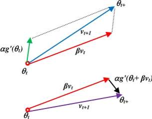
βwith 0 <  < 1 is the momentum term. At the beginning of the iteration process, the velocity is assumed to be zero (v0 = 0). The top part of Figure 4 illustrates the update rule of the standard momentum gradient descent. The blue vector represents the direction to adjust the parameters.

Assuming that the accumulated velocity β∙ vt will result in a move that reduces the value of the function to be optimized, it would seem to be a better choice to determine the gradients after applying the accumulated velocity. That is, one determines new parameter values by t+1/2 t - β∙vt , and then uses the gradient at position t+1/2, g'(t+1/2) rather than g'(t) for the final update. This is Nesterov's Accelerated Gradient (NAG, Nesterov, 1983) method, where the velocity vt+1 is determined according to:

vt+1 = β∙vt + t∙ g't - β∙vt) (3) This update rule is indicated by the lower part of Figure 4. The NAG method has been shown to be suitable for determining the parameters of deep neural networks in (Sutskever et al., 2013).

Figure 4. (Top) Momentum method and (Bottom) Nesterov's Accelerated Gradient (NAG) (Sutskever et al., 2013).

An alternative to avoid oscillating behaviour of gradient descent is given by the rmsprop method (Hinton et al., 2016), in which the gradient is normalised by the average gradient magnitude. overlapping subsets (the mini-batches), and each mini-batch is used to update the parameters once per epoch. In each epoch m, the learning rate m remains unchanged; that is, we use t = m. As soon as epoch m is finished, the learning rate is updated according to m+1 = m∙decrease, and a new random division of the training data into mini-batches is carried out, which serves as the basis for the next epoch. In each epoch, the parameters are updated M times using the following steps:

1) For the current position t, apply the momentum by t+1/2 =

Note that the iteration counter t is incremented after processing each mini-batch, but it is not reset to 0 when a new epoch starts.

The learning algorithm in this paper is different from standard gradient decent because it starts with a guess by moving the current parameter to a new position t+1/2 with the accumulated gradients and momentum, followed by a correction (gradient calculation) at t+1/2 and an update according to that gradient. We also evaluate the loss on the validation set after each training epoch. If the loss does not decrease for three subsequent epochs, we stop the training process and record the parameters in the current epoch as optimized parameters. A performance comparison of the method in our paper and other training methods is present in section 4.2.

3.3.2 Gradient computation: The loss function is calculated

where (.) is an indicator function; it equals to 1 if the argument is true and 0 otherwise. The derivatives of the distance di with must be summed over the two subnets:

1 compare our method to other state-of-art descriptor learning techniques.

4.1 Experimental Data and Setup

Our experiments are based on the Brown dataset (Brown et al., 2011) is used. This dataset is widely used in descriptor learning studies, e.g. (Trzcinski et al., 2012; 2015; Han et al., 2015; Zagoruyko and Komodakis, 2015). The dataset contains three separate subsets - Notre Dame (ND), Yosemite (Yos) and Statue of Liberty (Lib). All patches were extracted in the vicinity of Difference of Gaussian (DoG) feature points on real multi-view

t

images. Thus, real viewpoint changes are contained in those datasets. The original patch size is 64 x 64 pixels. The resize these patches to 32 x 32 pixels with anti-aliasing since the input of our model is designed as 32 x 32 pixels. Figure 5 gives some examples of the training pairs from the Notre Dame dataset (Brown et al., 2011).

Figure 5. Examples for training pairs. The left three columns are positive (matching) training pairs and the right three columns are negative (non-matching) training pairs.

The hyper-parameters for training were chosen empirically. In detail, we trained in 30 epochs and 450 mini-batches are used for training. Other parameters used here areβ = 0.9,γ = 0.9, α = 0.003, αdecrease = 0.9, lpull = 5, lpush = 10. Each mini-batch contains 500 positive and 500 negative training samples.

4.2 Convergence Behaviour

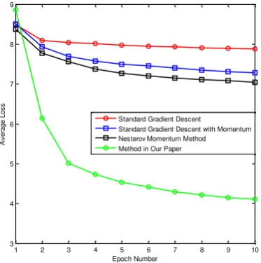
In this section we compare the convergence behaviour of our training method to standard gradient decent, gradient decent with momentum and to gradient decent with Nesterov's momentum. In this comparison, the same 50000 positive and 50000 negative training samples from the Notre Dame dataset were used for all four training methods in 10 epochs. The learning rate and the momentum term were set to the values described in section 4.1. The results are presented in Figure 6. The figure shows that the decrease of loss does not benefit too much from using only gradient descent or gradient descent with momentum; however, the training benefits distinctly from moving average gradients combined with the NAG (green curve in Figure 6), which obviously leads to a much faster decrease of the loss function.

1 2 3 4 5 6 7 8 9 10

3 4 5 6 7 8 9

Epoch Number

A

v

e

ra

g

e

L

o

s

s

Standard Gradient Descent

Standard Gradient Descent with Momentum Nesterov Momentum Method Method in Our Paper

Figure 6. Results of loss function for standard gradient descent, standard gradient descent with momentum, NAG and the method suggested in this paper.

4.3 Results and evaluation

In the set of experiments reported in this section, the descriptor is trained using one of the three datasets, whereas the other two datasets are used as for testing. This experiment was repeated three times, so that each dataset was used for training once. Each dataset contains 250,000 positive and 250,000 negative training pairs. The cross validation set consisted of 25,000 matching pairs and 25,000 non-matching pairs that were randomly selected from the dataset. Thus, the number of patch pairs used for gradient descent was 450,000 in each experiment. The cross validation set was used to determine the loss after each epoch in order to evaluate the stopping criterion: When the loss measured did not improve for three subsequent epochs, the training process was stopped.

To implement the whole architecture building and learning algorithm explained in section 3, we used the matconvnet software1 (Vedaldi and Lenc, 2014) to conduct the convolution, pooling, sigmoid and back-propagation of the basic CNN layers. The overall training procedure of the Siamese model is based on our own implementation. It runs on a 8-core 3.40Ghz CPU; training for one dataset takes about 11 hours.

For each training dataset, the performance test is evaluated on the other two datasets, which is a standard evaluation rule, also suggested in (Brown et al., 2011). In each test dataset, all the positive and negative examples are used as evaluation dataset. The evaluation criterion is the false positive rate at 95% recall rate. A lower false positive rate at 95% recall rate means better performance.

After training, the descriptors for each patch in the test datasets are determined using the parameters learned with the CNN. Then, the L2 Norm of the two descriptors of each test pair is computed as the similarity measure of the patch pair. A patch pair with an L2 Norm below a threshold h is classified to be a match, otherwise it is judged as a non-match. Thus, in essence, the learned descriptor can be considered to be a direct replacement of SIFT. As the true labels (match or non-match) of all patch pairs are known, the true positive and false positive rate can be calculated. By varying the threshold h a ROC curve is generated. The vl_roc function in the vlfeat2 software is used to obtain the ROC curve of the false positive rate against the true positive rate.

Table 2 lists the results of our work, comparing them to several state-of-art methods. None of the methods compared in the table contains a decision layer, i.e., a classifier to determine the matching label (matched or unmatched). The list constitutes a comparison of current state-of-art methods for descriptor learning. In the method SIM (Simonyan et al., 2014), learning is based on a convex optimization strategy. The learning procedure is an extension of method BR (Brown et al., 2011), which is a benchmark in descriptor learning. For method TRC (Trzcinski et al., 2015), we chose their best performing descriptor variant for our comparison, which is the floating point version with 64 bits. In method OS (Osendorfer et al., 2013), a descriptor learning architecture based on a Siamese CNN similar to our work was used, but the authors concentrated more on the comparison of different forms of loss functions and their model is trained by standard gradient descent. Finally, SIFT (Lowe, 2004) is used as a general baseline for the

1

http://www.vlfeat.org/matconvnet/ (accessed 05 April 2016)

2 _{http://www.vlfeat.org/ (accessed 05 April 2016)} ISPRS Annals of the Photogrammetry, Remote Sensing and Spatial Information Sciences, Volume III-3, 2016

descriptor matching, because it is widely acknowledged as a good descriptor in a feature engineering manner.

Among the six combinations of training and test dataset cases, our method and (Simonyan et al., 2014) achieve the best results in three cases each. For the mean error rate at 95% recall, our method is slightly worse but compatible with (Simonyan et al., 2014). Our method exceeds the best descriptor variant in (Trzcinski et al., 2015), namely FPBoost512-{64}, in terms of error rate at 95% recall in all training and test data combinations and a performance improvement of nearly 7.1% is achieved. To the best of our knowledge, Osendorfer et al. (2013) published the best results for a method for descriptor learning based on Siamese CNN architecture without classifier so far; it is the method most similar to ours in our comparison. Compared to this method, we achieved a performance improvement of 3.5%. Compared to SIFT, our method, as well as the other machine learning based descriptors, shows a distinct improvement in terms of the error rate at 95% recall.

Some of the randomly selected true positive, false positive, true negative and false negative patch pairs are shown in figure 7. To pick those patch pairs, the parameters are trained from the Statue of Liberty training data and the selected results are all from the Notre Dame dataset.

True Positive Pairs True Negative Pairs

False Positive Pairs False Negative Pairs

Figure 7. Some results of test on Notre Dame dataset.

5. CONCLUSIONS

In this paper we describe training of a descriptor based on a Siamese CNN architecture. In comparison to other work based on Siamese CNN, we use a more advanced gradient descent training algorithm and take a smaller input patch size. Our work demonstrates that with advanced training strategies, descriptors based on Siamese CNN achieve state-of-art performance on the Brown dataset.

When applied to real image matching or image retrieval, a feature descriptor needs to be matched against thousands of others. Therefore, as an extension of our work we will adapt the method by adjusting the proportion of positive and negative training samples that the model sees during training. Another extension includes applying this architecture to train descriptors that are able to cope with specific situations like oblique aerial images which contain more complex geometric transformations.

ACKNOWLEDGEMENTS

The author Lin Chen would like to thank the China Scholarship Council (CSC) for financially supporting his PhD study at Leibniz Universität Hannover, Germany.

REFERENCES

Aanæs, H., Dahl, A. L., Pedersen, K. S., 2012. Interesting interest points. International Journal of Computer Vision, 97(1), pp. 18-35.

Bay, H., Ess, A., Tuytelaars, T., et al., 2008. Speeded-up robust features (SURF). Computer Vision and Image Understanding, 110(3), pp. 346-359.

Beis, J. S., Lowe, D. G., 1997. Shape indexing using approximate nearest-neighbour search in high-dimensional spaces. In Proceedings of the IEEE Conference on Computer Vision and Pattern Recognition, pp. 1000-1006.

Bengio, Y., Courville, A., Vincent, P., 2013. Representation learning: A review and new perspectives. IEEE Transactions on Pattern Analysis and Machine Intelligence, 35(8), pp. 1798-1828.

Bishop, C. M., 2006. Pattern recognition and machine learning. Springer, New York, pp. 241-245.

BMRL (Biomimetic Robotics and Machine Learning Group, TU Munich, Germany), 2013. rmsprop.

https://climin.readthedocs.org/en/latest/rmsprop.html (accessed 05 April 2016)

Bromley, J., Bentz, J. W., Bottou, L., Guyon, I., LeCun, Y., Moore, C., & Shah, R., 1993. Signature verification using a “Siamese” time delay neural network. International Journal of

Training Test Ours SIM BR TRC OS SIFT

ND Yos 11.6 10.1 13.6 15.9 15.3 29.2

ND Lib 11.6 12.4 16.9 17.9 14.6 36.3

Lib ND 6.4 7.2 - 14.7 10.1 28.1

Lib Yos 11.3 11.2 - 20.9 17.6 29.2

Yos ND 8.4 6.8 18.3 14.8 9.5 28.1

Yos Lib 14.4 14.6 12.0 22.4 17.6 36.3

Mean 10.6 10.4 15.2 17.8 14.1 31.2

Table 2. False positive rate [%] at 95% recall rate for the different methods being compared in this work using different training and test data subset combinations (ND: Notre Dame, Lib: Statue of Liberty, Yos: Yosimite). Compared methods: SIM (Simonyan et al., 2014); BR (Brown et al., 2011); TRZ (Trzcinski et al., 2015); OS (Osendorfer et al., 2013), SIFT (Lowe, 2004).

Pattern Recognition and Artificial Intelligence, 7(04), pp., 669-688.

Brown, M., Hua, G., Winder, S., 2011. Discriminative learning of local image descriptors. IEEE Transactions on Pattern Analysis and Machine Intelligence, 33(1), pp. 43-57.

Chen L., Rottensteiner F., Heipke, C., 2015. Feature descriptor by convolution and pooling autoencoders. In: The International Archives of Photogrammetry, Remote Sensing and Spatial Information Science, 40(3), pp. 31-38.

Carlevaris-Bianco, N., Eustice, R. M., 2014. Learning visual feature descriptors for dynamic lighting conditions. In International Conference on Intelligent Robots and Systems (IROS 2014), pp. 2769-2776.

Hadsell, R., Chopra, S., LeCun, Y., 2006. Dimensionality reduction by learning an invariant mapping. In Proceedings of the IEEE Conference on Computer Vision and Pattern Recognition, Vol. 2, pp. 1735-1742.

Han, X., Leung, T., Jia, Y., Sukthankar, R., Berg, A. C., 2015. MatchNet: Unifying Feature and Metric Learning for Patch-Based Matching. In Proceedings of the IEEE Conference on Computer Vision and Pattern Recognition. pp. 3279-3286.

Hinton, G., Srivastava, N., Swersky, K., 2016. Neural networks for machine learning - Lecture 6e: rmsprop. http://www.cs.toronto.edu/~tijmen/csc321/slides/lecture_slides_ lec6.pdf (accessed 05 April 2016)

Jahrer, M., Grabner, M., and Bischof, H., 2008. Learned local descriptors for recognition and matching. In Computer Vision Winter Workshop. Vol. 2. Moravske Toplice, Slovenia.

LeCun, Y., Bottou, L., Bengio, Y., Haffner, P., 1998. Gradient-based learning applied to document recognition. Proceedings of the IEEE, 86(11), 2278-2324.

Lin, T. Y., Cui, Y., Belongie, S., Hays, J., Tech, C., 2015. Learning Deep Representations for Ground-to-Aerial Geolocalization. In Proceedings of the IEEE Conference on Computer Vision and Pattern Recognition, pp. 5007-5015.

Lowe, D. G., 2004. Distinctive image features from scale-invariant keypoints. International Journal of Computer Vision, 60(2), pp. 91-110.

Nesterov, Y., 1983. A method of solving a convex programming problem with convergence rate O (1/k2). In Soviet Mathematics Doklady, 27(2), pp. 372-376.

Mikolajczyk, K., Schmid, C., 2005. A performance evaluation of local descriptors. IEEE Transactions on Pattern Analysis and Machine Intelligence, 27(10), pp. 1615-1630.

Moreels, P., & Perona, P., 2007. Evaluation of features detectors and descriptors based on 3d objects. International Journal of Computer Vision, 73(3), 263-284.

Morel, J. M., & Yu, G., 2009. ASIFT: A new framework for fully affine invariant image comparison. SIAM Journal on Imaging Sciences, 2(2), 438-469.

Osendorfer, C., Bayer, J., Urban, S., van der Smagt, P., 2013. Convolutional Neural Networks learn compact local image descriptors. In Neural Information Processing, Springer Berlin Heidelberg, vol. 8228, pp. 624-630.

Rumelhart, D. E., Hinton, G. E., Williams, R. J., 1986. Learning representations by back-propagating errors. NATURE, 323(9), pp. 533-536.

Simonyan, K., Vedaldi, A., Zisserman, A., 2012. Descriptor learning using convex optimisation. In: European Conference on Computer Vision, pp. 243-256.

Simonyan, K., Vedaldi, A., Zisserman, A., 2014. Learning local feature descriptors using convex optimisation. IEEE Transactions on Pattern Analysis and Machine Intelligence, 36(8), 1573-1585.

Sutskever, I., Martens, J., Dahl, G., Hinton, G., 2013. On the importance of initialization and momentum in deep learning. In Proceedings of the 30th _{international conference on machine} learning (ICML-13), pp. 1139-1147.

Tola, E., Vincent, L., Fua, P., 2010. Daisy: An efficient dense descriptor applied to wide-baseline stereo. IEEE Transactions on Pattern Analysis and Machine Intelligence, 32(5), pp. 815-830.

Trzcinski, T., Christoudias, M., Lepetit, V. and Fua, P., 2012. Learning image descriptors with the boosting-trick. Advances in neural information processing systems, In Advances in neural information processing systems, pp. 269-277.

Trzcinski, T., Christoudias, M., Lepetit, V., 2015. Learning image descriptors with boosting. IEEE Transactions on Pattern Analysis and Machine Intelligence, 37(3) pp. 597-610.

Vedaldi, A., Lenc, K.. 2015. MatConvNet-convolutional neural networks for MATLAB. In Proceedings of the 23rd Annual ACM Conference on Multimedia Conference, pp. 689-692.

Zagoruyko, S., Komodakis, N., 2015. Learning to compare Image Patches via Convolutional Neural Networks. In Proceedings of the IEEE Conference on Computer Vision and Pattern Recognition,pp. 4353-4361.

Zbontar, J., LeCun, Y., 2015. Computing the stereo matching cost with a Convolutional Neural Network. In Proceedings of the IEEE Conference on Computer Vision and Pattern Recognition, pp. 1592-1599.