REAL-TIME BLOB-WISE SUGAR BEETS VS WEEDS CLASSIFICATION FOR
MONITORING FIELDS USING CONVOLUTIONAL NEURAL NETWORKS
Andres Milioto, Philipp Lottes, Cyrill Stachniss
Institute of Geodesy and GeoInformation, University of Bonn, Germany (andres.milioto,philipp.lottes,cyrill.stachniss)@igg.uni-bonn.de
KEY WORDS:Agriculture Robotics, Convolutional Neural Networks, Deep Learning, Computer Vision, Unmanned Aerial Vehicles
ABSTRACT:
UAVs are becoming an important tool for field monitoring and precision farming. A prerequisite for observing and analyzing fields is the ability to identify crops and weeds from image data. In this paper, we address the problem of detecting the sugar beet plants and weeds in the field based solely on image data. We propose a system that combines vegetation detection and deep learning to obtain a high-quality classification of the vegetation in the field into value crops and weeds. We implemented and thoroughly evaluated our system on image data collected from different sugar beet fields and illustrate that our approach allows for accurately identifying the weeds on the field.
INTRODUCTION
Agrochemicals can have several side-effects on the biotic and abi-otic environment and may even harm human health. Therefore, we need better tools and novel approaches to achieve a reduction in the use of agrochemicals in our fields. In conventional weed control, the whole field is treated uniformly with a single herbi-cide dose, spraying the soil, crops, and weed in the same way. In order to perform selective spraying, we must acquire knowl-edge about the spatial distribution of the weeds and plants in the field. One way to collect this data is through UAVs equipped with vision sensors in combination with an automatic classifica-tion system that can analyze the image data and label the crops as well as the weeds in the acquired images. One could even go a step further and use autonomous ground vehicles to execute a me-chanical or laser-based elimination of the individual weed plants identified by the UAV.
In this paper, we address the problem of classifying image content into crops and weeds. By exploiting the georeferenced location of the UAV, the location for each plant can be determined using a bundle adjustment procedure. Through a detection on a per-plant basis of sugar beets (crops) and typical weeds, we can select rele-vant information for the farmers or for instructing an agricultural ground robot operating on the field. Given the 3D information and a pixel-wise labeling of the images obtained with our ap-proach, we can directly provide the location of every weed to a ground robot or to a selective spraying tool used on a traditional GNSS-controlled tractor.
Thus, we focus in this paper on the vision-based classification system for identifying sugar beet plants and weeds. We rely on RGB and near infra-red (NIR) imagery of agricultural fields (see Figure 1 for an example). We use modern convolutional neural networks and deep learning pipelines to separate the plants based on their appearance. Our approach is an end-to-end approach, i.e., there is no need to define features for the classification task by hand.
The main contribution of this paper is a vision-based classifica-tion system to separate value crops from weeds using convolu-tional neural networks (CNNs). We target sugar beets as crops,
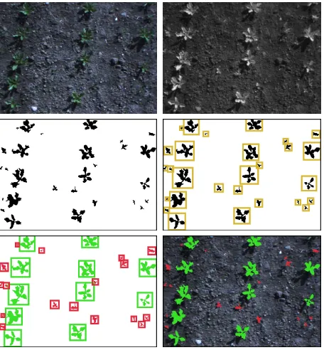
Figure 1. Illustration of our approach. Top: Original RGB and NIR images. Middle: NDVI mask and connected blob segmentation. Bottom: Classified blobs and pixel-wise overlay
to original image.
images. Furthermore, the network can be executed in real-time in a UAV.
In sum, we make the following four key claims: Our approach (i) does not require any hand-crafted features and thus can be imple-mented quickly, (ii) is able to provide accurate weed classification in real sugar beet fields with an accuracy of more than 95% in a field with plants in similar growth stage, (iii) can be retrained ef-ficiently to reuse the learned features for other data types or later growth stages, and (iv) is lightweight and fast, which makes it suitable for online operation in a flying robot.
RELATED WORK
The ability to estimate semantic information from sensor data is an important capability for autonomous and semi-autonomous systems operating indoors (Stachniss et al., 2005) as well as out-doors (Lottes et al., 2016a). For example, mobile robots like UAVs and ground vehicles serve as sensor platforms to obtain fast and detailed information of arable field environments. Robotic approaches for monitoring key indicators of crop health have be-come a popular research topic. Geipel et al. (2014), Khanna et al. (2015), and Pfeifer et al. (2016) estimate the crop height as well as the canopy cover using UAV imagery. These works rely on bundle adjustment procedures to compute terrain models and subsequently perform a vegetation segmentation to estimate the crop height based on the obtained 3D information.
Several approaches have been developed for vision-based vegeta-tion detecvegeta-tion by using RGB as well as multispectral imagery of agricultural fields (Guo et al., 2013; Hamuda et al., 2016; Torres-Sanchez et al., 2015). Hamuda et al. (2016) present a survey about plant segmentation in field images by analyzing several threshold based as well as learning based methods. Torres-Sanchez et al. (2015) investigate an automatic and adaptive thresholding method for vegetation detection based on the Normalized Difference Veg-etation Index (NDVI) and the Excess Green Index (ExG). They report a vegetation detection rate of around90−100%. In con-trast, Guo et al. (2013) apply a learning-based approach using a decision tree classifier for vegetation detection. They exploit spectral features using different color spaces based on RGB im-ages to perform a prediction on a per-pixel basis.
In the context of leaf image classification and segmentation, re-searchers have investigated using hand-crafted features and struc-tural operators (Wang et al., 2008; Kumar et al., 2012; Cerutti et al., 2013; Elhariri et al., 2014). Wang et al. (2008) segment leaf images by using morphological operators and shape features and apply a moving center hypersphere classifier to infer the plant species. Kumar et al. (2012) start from segmented images of leaves. They extract curvature features and compare them with a given database to find the best match with a labeled type. To cover a variety of leaf shapes, Cerutti et al. (2013) apply a de-formable leaf model and use morphological descriptors in order to classify their species. Elhariri et al. (2014) compare a Ran-dom Forest classifier and a linear discriminant analysis based ap-proach in their work for classifying 15 plant species by analyzing leaf images. They extract statistical features from the HSV color space of leaf images as well as gray level co-occurrence matrices to exploit additionally shape and vein (leaf structure) information. Hall et al. (2015) conducted a study on features for leaf classifi-cation. They compared the classification performance based on classical hand-crafted and ConvNet features by using a random forest classifier. They simulated varying conditions on the public
Flavia leaf dataset and conclude that ConvNet features support the performance and robustness of the classification results.
In contrast, we avoid the time consuming process of designing features by hand and exploit a CNN approach in order to com-pletely learn a representation of the data, which is suitable for discriminating sugar beets and weeds in image patches.
In the field of machine learning, several approaches have been ap-plied to classify crops and weeds in imagery of plantation (Garcia-Ruiz et al., 2015; Guerrero et al., 2012; Perez-Ortiz et al., 2016, 2015; Haug et al., 2014; Lottes et al., 2016a, 2017; Latte et al., 2015). Perez-Ortiz et al. (2015) propose an image patch based weed detection system. They use pixel intensities of multispec-tral images and geometric information about crop rows in order to build features for the classification. They achieve overall accu-racies of75−87% for the classification by analyzing the perfor-mance of different machine learning algorithms. Perez-Ortiz et al. (2016) use a support vector machine classifier for crop/weed detection in RGB images of sunflower and maize fields. They exploit statistics of pixel intensities, textures, shape and geomet-rical information as features. Guerrero et al. (2012) propose a weed detection approach for image data containing maize fields. Their method allows to identify the weeds after its visual appear-ance changed in image space due to rainfall, dry spell or herbicide treatment. Garcia-Ruiz et al. (2015) propose an approach for sep-arating sugar beets and thistle based on narrow band multispec-tral image data. They apply a partial least squares discriminant analysis for the classification and obtain a recall of84% for beet and 93% for thistle by using only four of the narrow bands at
521,570,610and658nm. Haug et al. (2014) present a method to detect carrot plants in weeds by using RGB and NIR-images without needing a presegmentation of the scenes into vegetation blobs. They perform a prediction on pixel level on a sparse grid in image space and report an average accuracy of around 94% on an evaluation set of70images where both, intra and inter-row overlap is present. In previous work, Lottes et al. (2016a, 2017) design a crop and weed classification system for ground and aerial robots. The work exploits NDVI and ExG indices to first segment the vegetation in the image data and then applied a random forest classifier to the vegetative parts to further dis-tinguish them into crops and weeds. Latte et al. (2015) use color space features and co-occurrence matrices to classify images cap-tured on crop fields containing several plant types. They apply an artificial neural network classifier and obtain an accuracy around 84% on average. Their results show that using statistical mo-ments of the HSV distribution improves the overall classification performance.
problem by using an end-to-end ensemble of CNNs. They ob-tain these lightweight CNNs through the compression of a pre-trained, more descriptive and complex model, and report an ac-curacy of 93.9%, processing images at little over 1 frame per second. Potena et al. (2016) present a perception system based on RGB+NIR imagery for crop and weed classification using two different CNN architectures. A shallow network performs the vegetation detection and then a deeper network further dis-tinguishes the detected vegetation into crops and weeds. They perform a pixel-wise classification followed by a voting scheme to obtain predictions for detected blobs in the vegetation mask. They obtain a performance of around97% for the vegetation de-tection, which is comparable to a threshold based approach based on the NDVI, and98% for the crop and weed classification in case the visual appearance has not changed between training and testing phase.
Our approach uses RGB-NIR imagery and CNNs, and is able to reach an accuracy of 97% with low running times even in embed-ded hardware that can be fitted in a flying platform. We achieve 97% precision and 98% recall for the classification of the weeds when the classifier is used in a similar growth stage as the one it was trained in. We are also able to obtain 99% recall and 89% precision for weeds in later growth stages without retraining. Fi-nally, we show that we can jump from 89% to 97% in recall for weeds if we retrain the classifier with new data from the current growth stage in a fast way. All of this allows our system to do statistics and selective weed removal in a very quick and accurate manner.
VISION BASED PLANT AND WEED CLASSIFICATION
The main goal of our plant classification pipeline is to allow mo-bile agricultural robots to detect unwanted species to remove them reactively, by either applying selective spraying or mechanical extraction/destruction. This requires the algorithm to run in real-time (or near real-real-time) on hardware that is compact and light enough to run in a flying platform, which is our principal aim. In our case, we consider the case of sugar beet plantations, which is a valuable study case both due to its popularity in Northern Europe, and because it has been solved before using other ap-proaches, which gives us the possibility to compare accuracy, ro-bustness and real-time capabilities against other state-of-the-art algorithms.
We need to achieve a high recall on the weed classification in or-der to enable the robot to remove a high number of weeds on the field. Therefore, we detect the coordinates relative to the robot’s coordinate system to synchronize the removal with the extrac-tion/spraying systems. This means that we are relaxed on the boundaries of the plants as long as we are able to direct the re-moval tools to the right position within our desired accuracy with-out harming the valuable crops. This allows for certain hypothe-ses that make a computationally cheap and fast blob approach suitable while still achieving state-of-the-art performance, such as: doing most of the training of the classifier and weed removal in early stages of the crop growth, and relaxing on the precision of the boundaries of the vegetation at the pixel level. However, as we can see in the last image of Figure 1, where the output classification is overlayed with the input image, a combination of the NDVI thresholded segmentation with a blob segmentation and classification gives a solid almost pixel-wise representation of the output mask, due to the masking done by the preprocess-ing, making this algorithm not only faster but also very similar in
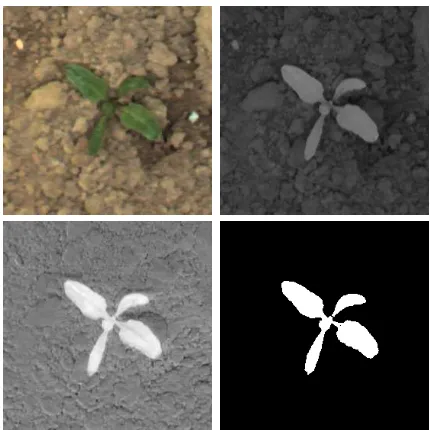
Figure 2. Top: RGB and NIR images. Bottom: NDVI transform and mask obtained by a conservative threshold in the NDVI
image.
output quality as the pixel-wise approach, which is both compu-tationally more complex and more time expensive to label.
We divide our classification pipeline in three main steps. First, we perform a vegetation detection to eliminate irrelevant soil in-formation from the images using multispectral images containing RGB and near infra-red information. Second, we describe the detected vegetation with a binary mask and perform a blob seg-mentation in order to extract patches containing singular crops or weeds. Finally, we classify each patch with a convolutional neural network that we train in an early growth stage to avoid overlapping crops and weeds in the data, and that we can later on re-train in a supervised or semi-supervised manner to adapt to other types of crops, or other stages of the crop growth. The blob approach makes the network run fast for both the forward pass and the retraining of the classifier, which makes it able to run on a flying platform using readily available single-board computers such as the NVIDIA Jetson platform. In the following subsec-tions we discuss each step of the pipeline in more detail.
Vegetation Detection
The goal of this pre-processing step is to separate the relevant vegetation content of every imageItaken by the robot from the soil beneath it, for which we need to apply a mask of the form:
IV(i, j) =
1, ifI(i, j)∈vegetation
0, otherwise , (1)
with the pixel location(i, j).
as our mask, as we can also see in Figure 2. Namely, using the NDVI to create the mask we have:
INDVI(i, j) =
INIR(i, j)− IR(i, j)
INIR(i, j) +IR(i, j)
(2)
Such transformation is used successfully to solve this very prob-lem by Lottes et al. (2016b), and improved by Potena et al. (2016) by adding a low cost convolutional neural network to a mapping obtained by a very permissive thresholding in the post NDVI seg-mentation operation. In our experiments, we use the thresholded segmentation of the NDVI-transformed image, similar to Lottes et al. (2016b), to separate the plants from the soil. An example is shown in Figure 2.
A threshold-based classification based on the NDVI can also lead to individual pixel outliers (or small groups of pixels). These are mostly caused by lens errors as chromatic aberration, which leads to a slightly different mapping of the red and the near infra-red light on the camera chip. We eliminate most of these effects through basic image processing techniques such as: morpholog-ical opening and closing operations to fill gaps and to remove noise at contours, which is done with a 5×5 disk kernel 1× open-ing followed by a 1×closing; and removal of tiny blobs which share less than a minimum amount of vegetation pixels, which depends on the Ground Sampling Distance and therefore it varies with the UAV distance to ground.
Blob-wise Segmentation
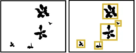
Given the vegetation mask we search for vegetation blobs. Each vegetation blob is given through a connected component of the vegetation pixels in the image (see Figure 3). We create an indi-vidual image patch of a certain size (64×64 pixels in our current setup) for each detected blob in the vegetation mask. Here, we first compute the bounding box of the contour of the blob and ap-ply an affine transformation to it in order to translate the blob into the center of the image patch and scale it to the desired size.
These image patches serve as input for our classification approach. Thus, the CNN can learn a representation based on such patches, which mostly describe whole plants or leaves. Through center-ing the blobs within the image patches we achieve translation in-variance and through scaling the detected blobs we reduce the influence of the plant size, which can vary a lot even for plants growing on the same field.
Figure 3. Blob selection from connected regions.
Classification using Convolutional Neural Networks
The advantage of using Convolutional Neural Networks for im-age classification is that they have the ability to learn features describing complex non-linear relations between dependent and independent variables by themselves, when given enough data.
This is not only useful for achieving a high classification accu-racy in a specific dataset, but also to later transfer that knowl-edge to other domains. Therefore, we can train the network with a high number of plants from different species under different weather and lighting conditions and then use the feature extrac-tors to cheaply train other classifiers for unseen species.
The main ideas behind weight sharing and CNNs were introduced in LeCun et al. (1989) and LeCun et al. (1998), and more recently brought back to public interest by Krizhevsky et al. (2012) where they exploited an efficient GPU implementation of the convolu-tion to break the ImageNet challenge benchmark at the time by an astounding 10% difference over their closest competitor, mak-ing them widely popular. They make the assumption that in im-age data, neighboring pixels are more correlated than pixels far away, therefore introducing the concept of local connectivity, al-lowing for less neuron wiring, which yields not only in better results, but also in less training and execution time. Today, deep convolutional neural networks are undoubtedly the most widely used approach for image classification, with it’s more novel fla-vors achieving top-5 classification errors in the test set of Ima-geNet as low as 3.57% (He et al., 2015), and 3.08% (Szegedy et al., 2016), outperforming the average human classification error which is around 5%.
The original architecture used by Krizhevsky et al. (2012) is com-parably shallow when measured against today’s state-of-the-art image classification networks, but we use a similar one to solve our classification problem, because it proves to have enough ex-pressiveness to describe our decision boundaries and has the ad-vantage that it is cheap to train and run in compact and low-power consumption hardware such as the one in a UAV.
Selection of the Architecture
The network has to be expressive enough to be able to describe the decision boundary between classes, but not too expressive as to overfit to our training data. This characteristic is set by the depth of the network, the amount of kernels in each convolutional layer and the amount of neurons in the fully connected ones. To choose our network size, we iterate starting with networks of a small number of filters per layer and of only one convolutional layer and one fully connected, and grow the network until we are almost able to overfit to a small sample of our dataset. After this, we further increase the expressiveness by adding more kernels to each convolutional layer and more neurons to the fully connected ones, and we train it again using our full training dataset. To avoid the bigger network to overfit to our training data we use a state-of-the-art method called “dropout” (Srivastava et al., 2014). This prevents neurons from learning complex co-adaptations in the fully connected layers by randomly dropping some of them during training, making the network generalize better, which we corroborate by getting a good performance in our cross-validation data. We also have to be careful to set an upper boundary in the network’s complexity, due to our constraint of real-time capabil-ity, meaning that the network needs to be both lightweight and of a complexity that is low enough to run fast in an embedded platform that we can fit in a flying vehicle. We are careful when choosing the depth and size of each layer to enforce this restric-tion.
Figure 4. Detailed architecture used for the blob-wise classification.
function, which convert the output of the network to a pseudo-probability distribution that works well for this problematic.
From this we design a network like the one in Figure 4. This ar-chitecture is composed by 3 convolutional layers (2 of kernel size 5×5 and the last one of 3×3 kernels), all of them using the Rec-tified Linear Unit for the non-linearity, which proves to speed up training considerably, and followed by 2×2 max-pooling for di-mensionality reduction. These 3 convolutional and max pooling layers are followed by 2 fully connected layers with 512 neurons each, which results in a 512-dimensional vector to be fed into the softmax layer that outputs the pseudo probability distribution we want as an output.
It is important to note that even though the network is shallow compared to the ones used by He et al. (2015); Szegedy et al. (2016), it is more complex and than those normally used for plant discrimination problems (Potena et al., 2016). However, due to the blob approach, the network doesn’t need to examine every pixel of the original input image, and it only runs one time per segmented patch, speeding up the process considerably.
Retraining for different crop growth stage
As the plants grow, they not only change their size, but also their shapes and colors, which means that we may not get the best re-sults if the growth stage is very different. In this case, the features extracted from the convolutional and fully connected layers may still be useful, so we can try to retrain the last layer of the net-work, which is the classifier, by feeding the network with a sam-ple of labeled data in the new growth stage. We will show that even though the classifier is very good without retraining, this technique can yield significant improvements, and can be done in a fast way due to the need to only train a linear classifier and in a small subset of the new data.
EXPERIMENTAL EVALUATION
The experiments are designed to show the accuracy and efficiency of our method and to support the claims made in the introduction that our classifier is able to (i) learn feature representations by itself and thus be implemented quickly, (ii) learn an accurate de-cision boundary to accurately discriminate plants and weeds with an accuracy of over 95%, being able to eliminate a majority of weeds with a minimal number of misclassified crops when tested in a similar growth stage; (iii) quickly improve after retraining by
using the previously learned features and adapting the last layer to a small subset of labeled new data; and (iv) run in real-time.
We implement the whole approach presented in this paper rely-ing on the Google TensorFlow library. This allows a new PhD student in the field of plant classification to perform the full im-plementation of the approach and its evaluation in slightly over two months (not including the acquisition time of the training and evaluation datasets), which supports our claim (i) that due to the self-learning of feature descriptors the pipeline can be imple-mented quickly.
Training of the Network
To train the network we use a dataset which we will call “Dataset A”, from Table 1. We split the dataset in 3, leaving 70% of it available to us for training, 15% for validation, and 15% for test after the whole pipeline was designed and trained, and therefore show how the network generalizes to unseen data. This dataset was captured with the plants in an early growth stage and it is quite balanced in it’s plants/weeds relation. We compare it with Dataset B from Table 1, which was captured 2 weeks later, in a more advanced growth stage, and we analyze the performance of the network.
Both datasets were captured using a JAI camera in nadir view capturing RGB+NIR images. For a typical UAV based monitor-ing scenario, not every image from the camera needs to be classi-fied, and one image per second is sufficient for real applications. Thus, we take images at1Hz, setting the upper bound for testing our real-time classification capabilities to 1 second per raw input image.
Parameter Dataset A Dataset B
no. images 867 1102
no. patches 7751 28389
no. crops 2055 2226
no. weeds 5696 26163
Pc/Pw 0.36 / 0.64 0.08 / 0.92
avg. patch/image 9 25
Table 1. Information about the datasets.
aiming for scale and translation invariance, and we further apply 64 even rotations to try to learn rotationally invariant features. After this we perform a per image normalization, which is also a common practice in learning to speed up the training.
Then we run the training using a cross-entropy cost function, which works well with the ReLU activations, along with a first order optimizer, which we use to minimize the cost by using stochastic gradient descent in batch sizes of 100. During training we reduce the learning rate by a third every 2 epochs to converge better the cost function’s minima, and we run until convergence is achieved.
The training takes 3 days in a low-cost NVIDIA GeForce GTX 940MX, which is not a top notch graphics card, and it is actu-ally less powerful than a currently available embedded platform like the Jetson TX2 which runs in a drone. This is critical if re-training is necessary, as we show later. If we use state of the art GPU’s for training, the process is cut short by an order of magni-tude, not only because of the difference in the floating operations per second, but also because the whole pipeline can be stored in GPU memory avoiding a bottleneck in the copying operations from system memory to GPU memory before each calculation. In Table 2 we show these differences. This further supports our claim (i) that the system can be implemented quickly, given the short training time even in a low-cost GPU.
Model Cores Arch. TFLOPs RAM
Titan Xp 3840 Pascal 12 12GB
Jetson TX2 SoC 256 Pascal 1.5 8GB
GTX 940MX 384 Maxwell 0.84 2GB
Intel i7 - - 0.04
-Table 2. Hardware comparison.
Performance of the Classifier
This experiment is designed to support our claim (ii) which states that we learn an accurate decision boundary to accurately dis-criminate plants and weeds with an accuracy of over 95%, being able to eliminate a majority of weeds with a minimal number of misclassified crops.
We now analyze the accuracy of the learned classifier and we evaluate its invariance to the crop growth. We tested the accuracy of our classifier in the test set (which only contains unseen data) of dataset A, and its accuracy in the test set of dataset B, when trained in A. We can see the results in Table 3:
Dataset Test set A Test set B
Accuracy 97.3% 89.2%
Table 3. Accuracy of the classifier trained in train set of A, and evaluated in Test set of A and B.
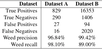
As we can see, we have a very high overall accuracy in the unseen data from dataset A, because it is from the same crop growth stage as the data the network has seen while it was being trained, and the performance of the classifier drops when used 2 weeks later. However, the overall accuracy does not say much about the quality of the classifier, especially in cases like dataset B, that are highly unbalanced. Since the main goal of our classifier is to detect weeds to proceed to their elimination, in Table 4 we show the obtained precision and recall for the detection of weeds in both datasets.
It is important to note that due to the nature of our problem it is critical to have a low precision in the weed classifier, because a large number of false positives means that plants get classified as weeds and thus get eliminated, especially in the case of me-chanical treatment. This is not the case for selective spraying, but spraying plants with herbicides defeats the purpose of the sys-tem anyway. It is also desirable to have a high recall to eliminate the most weeds we can, but not eliminating crops is of a critical importance.
Dataset Dataset A Dataset B
True Positives 829 16353
True Negatives 290 1406
False Positives 27 94
False Negatives 16 2020
Weed precision 96.84% 99.42% Weed recall 98.10% 89.00%
Table 4. Quality comparison of the classifier for the weed class trained in A.
Taking this into consideration, we can see from Table 4 that even if the recall of the weed detector decreases two weeks later, the precision is very high, allowing us to not eliminate valuable crops erroneously, fulfilling our demands for the system, and support-ing our claim (ii).
Retraining the network
This experiment is designed to prove claim number (iii) that our system can be easily and cheaply retrained to adapt to new growth stages.
As stated in the previous section, even though the precision of the weed detector was still very high two weeks later in the growth stage, the recall fell considerably, meaning that a good number of weeds were not being removed from the field. To fix this problem, we can cheaply retrain the last layer of the classifier, re-utilizing the feature vectors extracted by the convolutional filters learned from dataset A. We show the results it yields in Table 5, where we can see that both precision and recall have improved, mak-ing the system not only eliminate less crops erroneously, but also eliminate more weeds, which is the main purpose of it. In Table 6 we can also assess the general accuracy of the retrained classifier.
Dataset Trained in A Retrained in B
True Positives 16353 17927
True Negatives 1406 1190
False Positives 94 60
False Negatives 2020 696
Weed precision 99.42% 99.66%
Weed recall 89.00% 96.26%
Table 5. Quality comparison of the classifier for the weed class in test set of B, before and after retraining.
Dataset Trained in A Retrained in B
Accuracy 89.2% 96.1%
Table 6. Accuracy in dataset test set of B before and after retraining on small subset (15%) of training set of B.
This supports our claim that our system can be easily and cheaply adapted to new growth stages where plants have significantly changed their appearance.
Figure 5. Architecture used for the blob-wise classification, with the size of each layer specified and the amount of floating
operations needed per pass.
Runtime
This experiment is designed to prove claim number (iv) that our system can run in real-time in a flying platform. In Figure 5, we show another representation of the network, in which we can also see how many variables each layer contains, and how many float-ing operations it takes to pass through it. The final architecture needs 1.4 G floating point operations to do a full forward pass, which means that we can roughly calculate how long it will take to do a full pass depending on the FLOPs of the hardware. This results in Table 7. It is important to note that we left out the most powerful GPU because it is non realistic to think that we would put a desktop workstation in a small flying drone with the purpose of inference.
Another aspect we can see from Figure 5 is that the architecture is using a total number of 10 M 32-bit floating point parameters. This means that we can will have a full network size of 40 MB, which is something that our embedded hardware can store easily.
Hardware Theoretical time Actual time
Jetson TX2 SoC 1ms 4ms±1ms
Geforce GTX 940MX 2ms 7ms±1ms
i7 Processor 40ms 50ms±10ms
Table 7. Average and standard deviation running time per blob, depending on the hardware.
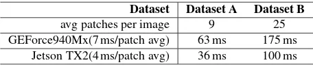
In Table 8, we analyze how long it would take in average to do a forward pass in all patches from a raw image, depending on the dataset. This highly depends on the growth stage, as we can see from the fact that dataset B has more patches per image, meaning that there are more plants and weeds present in the field, which makes sense. In this table we see that even with 25 images per image, which is our worst case, we are still very relaxed in our real-time constraint, by a margin of 5 in the case of our outdated GPU and a margin of 10 in the state of the art SoC, fulfilling our efficiency claim. This means that we can either analyze images at a higher frame rate, or fly higher, covering more crops, if the resolution of the camera is good enough to capture them from a distance. We also show that for our purposes, it is worth to loose
constant time complexity of the algorithm towards linear time be-cause, due to the upper bound of the number of patches contained in each raw image, we are actually gaining in performance.
Dataset Dataset A Dataset B
avg patches per image 9 25
GEForce940Mx(7 ms/patch avg) 63 ms 175 ms Jetson TX2(4 ms/patch avg) 36 ms 100 ms
Table 8. Average runtime per image.
As a final comment about runtime, we should consider that for each raw input image containingnvegetation blobs we segment we get a patch array of sizen. Since our neural network platform allows us to run forward passes in batch, we can gain a consider-able increase in performance if we send the whole batch of blobs to the GPU RAM at the same time, rather than queuing all oper-ations sequentially.
The presence of low cost, lightweight, power efficient hardware that can run this classifier in remarkably low time with great per-formances, make this approach a great alternative for online use in flying platforms working in dynamic environments. This sup-ports our claim number (iv) that our system can run in real-time in a UAV.
CONCLUSIONS
UAVs as well as other robots for precision farming must be able to distinguish the crops on the field from weeds. In this paper, we addressed the problem of detecting sugar beet plants and weeds using a RGB+NIR camera over real fields. We developed a classi-fication system based on convolutional neural networks (CNNs). Our approach is purely vision-based exploiting 4-channels and does not require geometric priors such as that the sugar beets must been planted in crop rows. In addition to that, the CNNs are an end-to-end approach such that no manual features must be de-fined. The input to the CNNs are blobs of vegetation and provide a classification output for such blobs. This renders the approach fast such that the system can be executed online. By relying on existing libraries for CNNs such as Tensorflow by Google, our classification system can be replicated quickly in the order of 2 months. We implemented our approach and thoroughly evalu-ated it using image data recorded on a real farm in different sugar beet fields and illustrate that our approach allows for accurately identifying the weeds on the field.
ACKNOWLEDGMENTS
This work has partly been supported by the EC under H2020-ICT-644227-FLOURISH and by the DFG under FOR 1505: Mapping on Demand. We would like to thank Chebrolu et al. (to appear) for providing part of the data used in our work.
References
Cerutti, G., Tougne, L., Mille, J., Vacavant, A. and Coquin, D., 2013. A model-based approach for compound leaves under-standing and identification. In:Proc. of the IEEE Int. Conf. on Image Processing (ICIP), pp. 1471–1475.
Chen, S., Skandan, S., Dcunha, S., Das, J., Qu, C., Taylor, C. and Kumar, V., 2017. Counting apples and oranges with deep learning: A data driven approach.IEEE Robotics and Automa-tion Letters.
Elhariri, E., El-Bendary, N. and Hassanien, A. E., 2014. Plant classification system based on leaf features. In: Computer Engineering Systems (ICCES), 2014 9th International Confer-ence on, pp. 271–276.
Garcia-Ruiz, F., Wulfsohn, D. and Rasmussen, J., 2015. Sugar beet (beta vulgaris l.) and thistle (cirsium arvensis l.) discrim-ination based on field spectral data. Biosystems Engineering 139, pp. 1–15.
Geipel, J., Link, J. and Claupein, W., 2014. Combined spectral and spatial modeling of corn yield based on aerial images and crop surface models acquired with an unmanned aircraft sys-tem.Remote Sensing6(11), pp. 10335.
Guerrero, J. M., Pajares, G., Montalvo, M., Romeo, J. and Gui-jarro, M., 2012. Support vector machines for crop/weeds iden-tification in maize fields. Expert Systems with Applications 39(12), pp. 11149 – 11155.
Guo, W., Rage, U. K. and Ninomiya, S., 2013. Illumination in-variant segmentation of vegetation for time series wheat im-ages based on decision tree model.Computers and Electronics in Agriculture96, pp. 58–66.
Hall, D., McCool, C., Dayoub, F., Sunderhauf, N. and Upcroft, B., 2015. Evaluation of features for leaf classification in challenging conditions. In: Applications of Computer Vision (WACV), 2015 IEEE Winter Conference on, pp. 797–804.
Hamuda, E., Glavin, M. and Jones, E., 2016. A survey of im-age processing techniques for plant extraction and segmenta-tion in the field.Computers and Electronics in Agriculture125, pp. 184–199.
Haug, S., Michaels, A., Biber, P. and Ostermann, J., 2014. Plant classification system for crop / weed discrimination without segmentation. In:Proc. of the IEEE Winter Conf. on Applica-tions of Computer Vision (WACV), pp. 1142–1149.
He, K., Zhang, X., Ren, S. and Sun, J., 2015. Deep residual learn-ing for image recognition.Computing Research Repository.
Khanna, R., M¨oller, M., Pfeifer, J., Liebisch, F., Walter, A. and Siegwart, R., 2015. Beyond point clouds - 3d mapping and field parameter measurements using uavs. In: Proc. of the IEEE Int. Conf. on Emerging Technologies Factory Automa-tion (ETFA), pp. 1–4.
Krizhevsky, A., Sutskever, I. and Hinton, G. E., 2012. Imagenet classification with deep convolutional neural networks. In: F. Pereira, C. J. C. Burges, L. Bottou and K. Q. Weinberger (eds),Advances in Neural Information Processing Systems 25, Curran Associates, Inc., pp. 1097–1105.
Kumar, N., Belhumeur, P. N., Biswas, A., W.Jacobs, D., Kress, W. J., L´opez, I. and Soares, J. V. B., 2012. Leafsnap: A com-puter vision system for automatic plant species identification. In:Proc. of the Europ. Conf. on Computer Vision (ECCV).
Latte, M. V., Anami, B. S. and B., K. V., 2015. A combined color and texture features based methodology for recognition of crop field image.International Journal of Signal Processing, Image Processing and Pattern Recognition8(2), pp. 287–302.
LeCun, Y., Boser, B., Denker, J. S., Henderson, D., Howard, R. E., Hubbard, W. and Jackel, L. D., 1989. Backpropagation applied to handwritten zip code recognition.Neural Computa-tion1(4), pp. 541–551.
LeCun, Y., Bottou, L., Bengio, Y. and Haffner, P., 1998. Gradient-based learning applied to document recognition. In: Proceed-ings of the IEEE, pp. 2278–2324.
Lottes, P., H¨oferlin, M., Sander, S. and Stachniss, C., 2016a. Ef-fective vision-based classification for separating sugar beets and weeds for precision farming.Journal on Field Robotics.
Lottes, P., H¨oferlin, M., Sander, S., M¨uter, M., Schulze-Lammers, P. and Stachniss, C., 2016b. An effective classifi-cation system for separating sugar beets and weeds for preci-sion farming applications. In:Proc. of the IEEE Int. Conf. on Robotics & Automation (ICRA).
Lottes, P., Khanna, R., Pfeifer, J., Siegwart, R. and Stachniss, C., 2017. Uav-based crop and weed classification for smart farm-ing. In:Proc. of the IEEE Int. Conf. on Robotics & Automation (ICRA).
McCool, C., Perez, T. and Upcroft, B., 2017. Mixtures of lightweight deep convolutional neural networks: Applied to agricultural robotics.IEEE Robotics and Automation Letters.
Mortensen, A. K., Dyrmann, M., Karstoft, H., J¨orgensen, R. N. and Gislum, R., 2016. Semantic segmentation of mixed crops using deep convolutional neural network. In: Proc. of the In-ternational Conf. of Agricultural Engineering (CIGR).
Perez-Ortiz, M., Pe˜na, J. M., Gutierrez, P. A., Torres-S´anchez, J., Herv´as-Mart´ınez, C. and L´opez-Granados, F., 2015. A semi-supervised system for weed mapping in sunflower crops using unmanned aerial vehicles and a crop row detection method. Applied Soft Computing37, pp. 533 – 544.
Perez-Ortiz, M., Pe˜na, J. M., Gutierrez, P. A., Torres-S´anchez, J., Herv´as-Mart´ınez, C. and L´opez-Granados, F., 2016. Selecting patterns and features for between- and within- crop-row weed mapping using uav-imagery.Expert Systems with Applications 47, pp. 85 – 94.
Pfeifer, J., Khanna, R., Dragos, C., Popovic, M., Galceran, E., Kirchgessner, N., Walter, A., Siegwart, R. and Liebisch, F., 2016. Towards automatic uav data interpretation for precision farming.Proc. of the International Conf. of Agricultural Engi-neering (CIGR).
Potena, C., Nardi, D. and Pretto, A., 2016. Fast and accurate crop and weed identification with summarized train sets for precision agriculture. In:Proc. of Int. Conf. on Intelligent Au-tonomous Systems (IAS).
Rouse, Jr., J. W., Haas, R. H., Schell, J. A. and Deering, D. W., 1974. Monitoring Vegetation Systems in the Great Plains with Erts.NASA Special Publication351, pp. 309.
Srivastava, N., Hinton, G., Krizhevsky, A., Sutskever, I. and Salakhutdinov, R., 2014. Dropout: A simple way to prevent neural networks from overfitting. Journal of Machine Learn-ing Research15, pp. 1929–1958.
Stachniss, C., Mart´ınez-Mozos, O., Rottmann, A. and Burgard, W., 2005. Semantic labeling of places. In: Proc. of the Int. Symposium of Robotics Research (ISRR).
Szegedy, C., Ioffe, S. and Vanhoucke, V., 2016. Inception-v4, inception-resnet and the impact of residual connections on learning.Computing Research Repository.
Torres-Sanchez, J., L´opez-Granados, F. and Pe˜na, J., 2015. An automatic object-based method for optimal thresholding in uav images: Application for vegetation detection in herbaceous crops.Computers and Electronics in Agriculture114, pp. 43 – 52.