AREA-BASED SNOW DAMAGE CLASSIFICATION OF FOREST CANOPIES
USING BI-TEMPORAL LIDAR DATA
M. Vastaranta*, I., Korpela, A., Uotila, A. Hovi, M. Holopainen
Department of Forest Sciences, University of Helsinki, Finland – [email protected]
KEY WORDS: Change detection, airborne laser scanning, logistic regression
ABSTRACT:
Multitemporal LiDAR data provide means for mapping structural changes in forest canopies. We demonstrate the use of area-based estimation method for snow damage assessment. Change features of bi-temporal LiDAR point height distributions were used as predictors in combination with in situ training data. In the winter 2009−2010, snow damages occurred in Hyytiälä (62°N, 24°E),
southern Finland. Snow load resulted in broken, bent and fallen trees changing the canopy structure. The damages were documented at the tree level at permanent field plots and dense LiDAR data from 2007 and 2010 were used in the analyses. A 5 × 5-m grid was
established in one pine−spruce stand and change metrics from the LiDAR point height distribution were extracted for the cells. Cells
were classified as damaged (n= 43) or undamaged (n = 42) based on the field data. Stepwise logistic regression detected the damaged cells with an overall accuracy of 78.6% (Kappa = 0.57). The best predictors were differences in h-distribution percentage
points 5, 35, 40, 50 and 70 of first-or-single return data. The tentative results from the single stand suggest that dense bi-temporal LiDAR data and an area-based approach could be feasible in mapping canopy changes. The accuracy of the point h-distribution is
dependent on the pulse density per grid cell. Depending on the time span between LiDAR acquisitions, the natural changes of the h
-distributions due to tree growth need to be accounted for as well as differences in the scanning geometry, which can substantially affect the LiDAR h-metrics.
1. INTRODUCTION
Snow is a natural element in the boreal forests of Finland that extend from 60° to 68°−70°N. During snow voluminous
winters, loads can reach over 1000 kg/crown (Jalkanen and Konopka 1998). The load on the trees consists of snow, rime and frozen sub cooled rain (Solantie 1980). The critical loads on the crown are achieved in special weather conditions common in regions which are higher than surrounding areas. The risk for low and moderate snow damage occurs, if the snow load on the crown exceeds 20−40 kg/m2 or the wind is heavy on
the same (Peltola et al. 1999). This limit is achieved every fifth year in Southern Finland and every third year in northern Finland (Solantie 1994).
Airborne LiDAR can be used for monitoring of the forest canopy structure. LiDAR-based forest inventory methods have been developed intensively in the last 6−12 years, and they are
currently gaining popularity (e.g. Naesset et al. 2004). The high geometric accuracy of the LiDAR observations lends support to assume that it is well suited for monitoring of forest dynamics. The same targets (stands, cells, trees) are observed with high reliability over time.
The general potential of LiDAR in forest monitoring applications is still largely unexplored (empirically), because LiDAR time-series that span more than a few years are but few. Bi-temporal LiDAR were used to monitor forest growth and intermediate fellings (Yu et al. 2004; St-Onge and Vepakomma 2004; Naesset and Gobakken 2005; Hopkinson et al. 2008; Yu et al. 2008). However, the short growth periods used (and slow growth of boreal trees) have resulted in low growth estimation accuracy. Undisturbed forest growth of dense or closed
cano-settings remain unchanged in multitemporal LiDAR data sets, the canopy changes should reduce pulse penetration to ground and increase the absolute values of upper height (h) distribution
percentiles. Changes in the acquisition settings affect the LiDAR observations even if the canopy remains unchanged. For example, different h-distributions are obtained by changing the
scan zenith angle from 0° to 20° with increasingly distorting effects at angles above 12°−15°. In area-based estimation of the
growing stock, which is typically done for stands, sub-stands, or grid cells, the stem volume estimates are derived indirectly using LiDAR point h-distribution metrics. Depending on the training data, the properties of the forest and the size of the observation unit, a standard error of 10−20% is typical for total
stem volume (Naesset et al. 2004). If for example the total stem volume is 250 m3/ha and the growth is 4−5 m3/ha/a, a long time period is required in order to have the standard error (SE) of the growth estimate below 10%. In this example, we assumed that the volume estimations of both time points are done indepen-dently. An alternative is to derive the change estimates by simultaneous analysis of the multitemporal LiDAR data in a given observation unit. Naesset and Gobakken (2005) observed statistically significant changes in bi-temporal LiDAR h
-metrics. However, the volume growth estimates had poor accuracy due to the 2-yr time interval between the LiDAR acquisitions. In temperate forests, Hopkinson et al. (2008) used multitemporal LiDAR data and concluded that even the annual forest h-growth was detectable. Similar to Næsset and
Gobakken (2005), the relative SE of the stand-level annual growth estimates were high (ca. 100%), but decreased rapidly when the time interval was extended (~10% after 3 years). Yu et al. (2004) studied the monitoring of intermediate fellings, which can be described as “sudden drastic canopy changes”, in which
suppressed trees. Intermediate felling can vary from light to heavy, and the selection of trees to be removed differs as well.
Our study concerns the detection of canopy changes due to snow damage using LiDAR h-distribution metrics. The changes
occurred between two high-density LiDAR acquisitions. A snow-damage means that entire tree stems are broken from various heights, some trees lose branches, and some trees become slanted. Foliage is “lost or repositioned”. In some sense snow-damage bears resemblance to an intermediate felling, except for the partially broken stems and slanted trees. Also, the selection of trees subject to removal is entirely different (spatial pattern, relative height of trees). Snow damage differs also from wind-induced changes, which are also common in Finland. In a bi-temporal LiDAR data set the changes due growth and insect damages etc. are also observable. The overall growth shows in increase of crown volumes, as seen from the above. It is evident that changes in the dominant tree layer are visible in LiDAR data, while changes in the lower canopy layer are more difficult to discern.
Our objective was to test the use of area-based change metrics in LiDAR point h-distributions in classifying snow-damage
induced canopy changes of different severity.
2. MATERIALS AND METHODS
2.1 Study area and field measurements
The study was conducted in Hyytiälä, southern Finland (61°50´N, 24°20´E). Hyytiälä hosts a multitude of permanent forest plots, and it has been scanned five times since 2004, using a small-footprint discrete-return LiDAR sensors. In 2009, a large number of the forest plots (16,000 trees) were measured to support ongoing remote sensing activities. Many of the forest plots were however subject to snow damage January−February
2010. The snow load started to accumulate in December 2009 continuing to February. General observations by the local fores-ters were that the most intensive damage occurred in high areas, where elevation exceeded 160 m above sea level and that the damage was more common in Scots pine forests. The SMEAR II research station in Hyytiälä is in a pine stand, where the rime and snow accumulation could be observed also in surveillance camera data (Fig. 1). In February the trees began to bend down. The snow load was mainly dropped in the end of February, when the temperature raised to 0°C with wind. Many trees were broken also then (Fig. 2).
In summer 2010, field work was carried out in pine-dominated plots that had been subject to different degree of snow damage in order to obtain reference data and to document the phenome-non. We used only one plot for this study (Table 1). The plot was established in 2005 and the tree maps were generated using a total station. Trees damaged by the snow were identified in the field in 2010. In addition, stem diameter (dbh) measurements
from 2009 were updated. There were broken, fallen and bent trees. Using existing data, it was possible to differentiate between an earlier damage and that from February 2010. The height of the broken stems was assessed visually. Tree heights were available for all trees from 2005 and 2009.
Fig. 1. Treetops (180−185 m a.s.l.) of a 50-year-old pine stand
in Hyytiälä, January 26, 2010 (Monitoring camera at the SMEAR II station).
Fig. 2. Broken stems and treetops at the field plot PS_TEX.
Table 1. Basic characteristics of plot PS_TEX (Autumn 2009).
Size, m 100 × 40
Age, years 65
Elevation, m 182.3
Mean height, Hg, m 21.0
Mean dbh, Dg, cm 23.9
Stem number, S, s/ha 840
Basal area, G, m2/ha 31.0
Stem volume, V, m3/ha 310
Vert. canopy cover % 62.7 Snow breaks, % 11.6 Partial snow breaks % 5.0
Bent % 0.5
PS_TEX represents a forest in the late thinning phase. The site quality of the plot is intermediate (Myrtillus type). Expected age for regeneration is 80−90 years depending in the thinning
regime. Plot was established by planting and is one of the oldest planted pine stands in the area
2.2 LiDAR data
The LiDAR data sets were acquired in 2007 and 2010, using airplane-mounted, topographic small-footprint discrete-return sensors (Table 2). In both acquisitions, the flight lines were oriented SSE−NNW and had 50−60% side overlap. The 2010
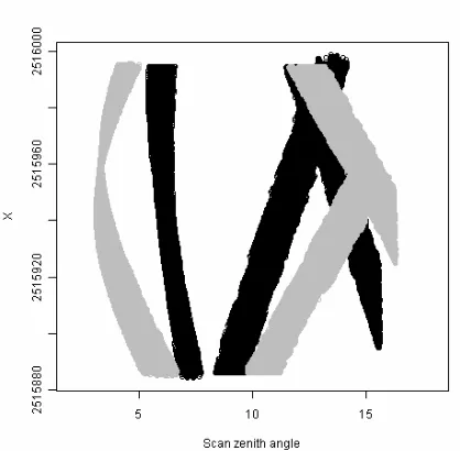
LiDAR sensor was equipped with waveform digitizer, but we used the discrete-return data. The ALS50-II and ALS-60 sensors use very similar sensor technology. LiDAR data from PS_TEX included areas covered by 2 or 3 flight. The scan zenith angle distributions per location varied between acquisitions (Fig. 3)..Plot PS_TEX was 100 × 40 m in area and
the wider, E−W-oriented side was perpendicular to the flight
lines of LiDAR.
Table 2. Sensor configurations in the LiDAR data sets.
Data set 2007 2010
Date July 4 July 19
Time, GMT 16−17:30 15−16
Instrument, Leica ALS50-II ALS60
Altitude, m, AGL 800 1000
Pulse frequency, kHz 116 174 Scanning frequency, Hz 52 68.4 Scanning angle (instrument) ±15° ±15°
Pulse density , m-2 7 11.9
Beam divergence (1/e), mrad 0.15 0.15 Automatic Gain Control, AGC yes yes
We used a digital elevation model (DEM) that was estimated from leaf-on LiDAR data of 2004 (1−2 pulses/m2, 1.3 km
height) It has been assessed to have an RMS-accuracy of 0.20−0.27 m in seedlings stands and closed-canopy forests.
Fig. 3. Scan zenith angle × X-coordinate scatterplots in plot
PS_TEX. Data from 2007 is drawn in grey, while 2010 is in black.
Raster format canopy height models (CHMs) were estimated from the 2007 and 2010 data for illustrations. The CHMs had
2.3 Extraction of area-based change features
In area-based analyses, the grid size defines the spatial sampling density. A small grid size is beneficial in the estimation of the spatial intrastand variation, but this comes at the expense of de-creased accuracy, because fewer pulses are available per cell. We considered snow damage a “discrete tree-level event”. The number of trees that belong to a grid cell of certain size depends on the stand density. In small cells, the damage of one tree has high proportional weight. However, the use of small cells also increases the total length of cell borders and cases, in which the crown (event) is split between cells. The pulse count depends on the cell size and the pulse density, but in a large cell, a single damaged tree does not contribute a substantial change. This shows that the choice of the cell size is challenging and probably should be adapted to local h variation that correlates
with stand density, at least in managed forests. Our dense LiDAR data enabled the use of the relatively small 25-m2 cell size. Given the density of 850 s/ha, there were on average two trees per cell.
Using field data, grid cells were defined a binary division into damaged (n=42) and undamaged (n=43) classes (Fig. 4). Damaged cells included crown projection area of damaged tree. Plot PS_TEX was not rectangular, and the border cells were omitted. Height percentiles at 5% (h5−h95, m) intervals
(20-quantiles) were calculated from the first-or-single return data of 2007 and 2010. Respective difference metrics in height percentiles ( h5− h95, m) were calculated.
Fig. 4. A 5-m grid in plot PS_TEX. Damaged cells were drawn in dark grey, while light grey depicts undamaged cells. The red crosses mark damaged trees and the black dots denote undamaged trees.
Snow damage affected the change of LiDAR point h
-distributions from 2007 and 2010 (Fig. 5). The pictured distributions comprise data from a single damaged and undamaged cell. In the undamaged case, the upper percentiles increased and the ground penetration percentage decreased 2007−2010. The three-year height growth of dominant trees is
approximately 0.75 m, and this is the difference of the h
-distribution maxima in 2007 and 2010. The damaged cell shows significantly different change pattern compared with the undamaged. The severe snow damage (one tree out of a
0 20 40 60 80 100
0
5
10
15
20
25
Percentile, %
Height, m
Undamaged 2010 Undamaged 2007 Damaged 2010 Damaged 2007
Fig 5. LiDAR h-percentiles in two 25-m2 m cells in 2007 and 2010.
2.4 Binary classification
Logistic regression (LR) can be used in binary classification problems. LR is commonly used in modelling the probability of an event’s occurrence. Here, we modelled the probability of the cell being snow damaged, using changes in the height per-centiles as predictors. In logistic regression, logit transformation is used to make the relationship between the response pro-bability and the predictor variables linear. The multiple logistic regression model is:
logit(p) = ln[p/(1-p)] = 0 + 1x1 + 2x2 +….+ nxn (1),
where p is the probability that an event will occur and x1…xn are the variables explaining the probability. The predicted probabilities are calculated by transforming back to the original scale:
p = exp(logit(p))/[1 + exp(logit(p))] (2)
For selecting the final predictors in the model, stepwise LR was applied with both forward and backward selections. The maximum number of steps to be considered was 1000 and the used multiple of the number of degrees of freedom for the penalty was log (n). R statistical package (R Development Core Team, 2007) was used in the analyses.
3. RESULTS
Fig. 6 shows how snow damage changes the point clouds in a vertical slice of LiDAR data. Fig. 7 illustrates the patterns in difference of canopy height surfaces and the effects to LiDAR point height distributions were seen in Fig. 5.
Fig 6. Slice of LiDAR data showing vertical profiles. Black and grey points denote the LiDAR data of 2010 and 2007, respectively. The 18-m-high co-dominant tree was broken at the h of 8 m.
Fig 7. Difference of CHMS, CHM2007−CHM2010 [m]. Dama-ged crowns are superimposed as circles. Positive differ-ence indicates decrease in h between 2007 and 2010.
Stepwise logistic regression detected the snow damaged cells with an overall leave-one-out cross-validation accuracy of 78.6% (Simple Kappa = 0.57). The selected predictors were
h5, h35, h40, h50, and h70.
4. DISCUSSION
We report a test about the use of change metrics calculated from dense bi-temporal LiDAR point h-distributions for area-based
detection of snow damages. Classification accuracy was 78.6% in a binary classification of damaged and undamaged cells. Based on our tentative results we can state that snow damages result in such structural canopy changes that can be observed in LiDAR data using an area-based approach. However, we did not do an elaborate analysis of the possible LiDAR predictors. Our data comprises of a single stand, and the density of the grid was also omitted in the analyses.
We had three growing seasons between the LiDAR acquisitions. Changes due to tree growth were also observable (Fig. 5), but not examined further here, because the proportional annual stem volume growth is only 2-3% in the studied forest. If the time period between LiDAR acquisitions is long, there can be more effects due to (height) growth, intermediate fellings and other factors. Separation of those from a non-recurrent damage will of course be impossible using our approach. We used a small, 5-m grid. With large grid cells, the ratio between the damaged and undamaged trees changes and for example the damage (low severity in a cell) of a single tree is easily obscured by the growth of other trees and other factors changing the LiDAR h-distributions. Another important factor
that is related to the used grid size is the applied pulse density. We had a dense, small-footprint LiDAR data, 7 to 12 pulses per m2. With a more sparse LiDAR data, larger grid size has to be used for stable and accurate measurements on the h
-distributions. Sensitivity of the area-based damage detection to cell size, and forest structure (and LiDAR acquisition settings) constitutes a future research topic.
In bi-temporal LiDAR data, there is always noise (imprecision of the h-distributions) caused by sampling
er-rors and scan geometry changes (Fig. 3), tree/branch move-ment, and geometric inaccuracy. Still, the relative high geo-metric reliability of airborne LiDAR data is very promising for monitoring applications in forestry.
Bi-temporal LiDAR data are not widely available and the acqui-sition costs for damage inventory only can become substantial if the spatial occurrence of the damage is sporadic and local (cf. snow damage). Our area-based method requires in situ data. For practical applications, more suitable method (with high-density LiDAR data) for canopy disturbance mapping could be based on difference imaging of the CHMs (Fig. 7). Snow damage is a local phenomenon that is related to topography, while severe storm damages occur at a larger scale. Large continuous areas are needed for cost-efficient LiDAR campaigns.
Changes in LiDAR h-metrics have been previously used to
monitor forest growth (Naesset and Gobakken 2005, Hopkinson et al. 2008, Yu et al. 2008). In this study bi-temporal LiDAR was tried in the detection of natural forest disturbancies. Although the tentative results were rather promising, damage classification (or canopy change detection) with area-based methods is far from practice. Data acquisition and field work costs need to be considered. The multitemporal LiDAR data
5. REFERENCES
Hopkinson, C., Chasmer, L. and Hall, R.J., 2008. The uncertainty in conifer plantation growth prediction from multi-temporal lidar datasets. RSE. 112, pp. 1168–1180.
Jalkanen, R. and Konôpka, B., 1998. Snow-packing as a poten-tial harmful factor on Picea abies, Pinus sylvestris and Betula using canopy metrics derived from airborne laser scanner data.
RSE. 96, pp. 453– 465.
Peltola, H., Kellomäki, S., Väisänen, H. and Ikonen, V-P., 1999. A mechanistic model for assessing the risk of wind and snow damage to single trees and stands of Scots pine, Norway spruce, and birch. Can. J. For. Res. 29, pp. 647-661.
R Development Core Team, 2007. R: A language and environment for statistical computing. R Foundation for Statistical Computing, Vienna, Austria. www.R-project.org.
Solantie, R., 1994. Effect of weather and climatological background on snow damage of forests in southern Finland in November 1991. Silva Fenn. 28, pp. 203-211.
Solantie, R. and Ahti, K., 1980. Säätekijöiden vaikutus Etelä-Suomen lumituhoihin v. 1959. Silva Fenn. 14, pp. 342-353.
St-Onge, B. and Vepakomma, U., 2004. Assessing forest gap dynamics and growth using multi-temporal laser-scanning data. Proceedings of the ISPRS working group VIII/2. ISPRS, Vol XXXVI, Part 8/W2, pp. 173-178,.
Yu, X., Hyyppä, J., Kaartinen, H. and Maltamo, M., 2004. Au-tomatic detection of harvested trees and determination of forest growth using airborne laser scanning. RSE. 90, pp. 451-462.
Yu, X., Hyyppä, J., Kaartinen, H., Maltamo, M. and Hyyppä, H., 2008. Obtaining plotwise mean height and volume growth in boreal forests using multi-temporal laser surveys and various change detection techniques. IJRS. 29, pp. 1367–1386.
ACKNOWLEDGEMENTS
Our thanks are due to Pauliina Kulha, Laura Kammonen, Anni Vanhatalo, Heli Miettinen, Piia Launiainen, Heidi Sjöblom, Isto Hongisto and Professor Eero Nikinmaa for the field work. The LiDAR data were made possible by a consortium of research and business partners. Work was funded by UH research funds, Academy of Finland, and Suomen Luonnonvarain tutkimussää-tiö.