STUDY ON MODELING AND VISUALIZING THE POSITIONAL UNCERTAINTY OF
REMOTE SENSING IMAGE
Weili Jiao*, Tengfei Long, Saiguang Ling, Guojin He
Institute of Remote Sensing and Digital Earth (RADI), Chinese Academy of Sciences, No.9 Dengzhuang South Road, Haidian District, Beijing 100094, China – (jiaowl, longtf, lingsg, hegj)@radi.ac.cn
Commission II, WG II/4
KEYWORDS: uncertainty, remote sensing, geometric correction, image quality, error model visualization
ABSTRACT:
It is inevitable to bring about uncertainty during the process of data acquisition. The traditional method to evaluate the geometric positioning accuracy is usually by the statistical method and represented by the root mean square errors (RMSEs) of control points. It is individual and discontinuous, so it is difficult to describe the error spatial distribution. In this paper the error uncertainty of each control point is deduced, and the uncertainty spatial distribution model of each arbitrary point is established. The error model is proposed to evaluate the geometric accuracy of remote sensing image. Then several visualization methods are studied to represent the discrete and continuous data of geometric uncertainties. The experiments show that the proposed evaluation method of error distribution model compared with the traditional method of RMSEs can get the similar results but without requiring the user to collect control points as checkpoints, and error distribution information calculated by the model can be provided to users along with the geometric image data. Additionally, the visualization methods described in this paper can effectively and objectively represents the image geometric quality, and also can help users probe the reasons of bringing the image uncertainties in some extent.
1. INTRODUCTION
A variety of complex factors, influence the remote sensing image to be positional geometric distortion during the image captured including atmospheric refraction, terrain distortions, and variation in orbit, etc. In order to integration with other spatial data, the imagery is usually geometric corrected and registered to standard coordinate systems. All these distorting influences and processing stages introduce spatial uncertainty to the data.
Positional accuracy of remote sensing image determines how closely the position of discrete objects shown on a geometric rectified image agrees with the true position on the ground. A standard method of assessing the positional accuracy is based on comparison of deviations between corresponding control points that can be accurately located on both the reference map and the geometrically corrected image. The deviations at these control points are used to compute statistics to evaluate the accuracy of the geometric corrected image, and in practice, the quantitative measure broadly used is the root mean square errors (RMSEs) of control points (Janssen & Van Der Wel, 1994, Buiten & Van Putten, 1997, Jiao, et al., 2008, Goncalves, et al., 2009, Vieira, et al., 2004, Long, et al., 2015). However, the RMSEs can only be used to evaluate the positional accuracy of the control points and not the accuracy of the overall image. Since the control points are individual and discontinuous, it is difficult to describe the error spatial distribution of the image. On the other hand the accuracy of the ground control points (GCPs) used for image rectification has been ignored in the evaluation of the image positional accuracy (Bastin, et al., 2002). It also should be noted that when so called geo-coded satellite imagery, processed through geometric rectification, is delivered to the user, the uncertainties are propagated (Arnoff, 1985, Ge, et al., 2006), including positional uncertainties of GCPs, DEM data, and the positional model, etc. So it is important to explore the methods of representing the positioning uncertainty of remotely sensed
imagery, and the information about data quality should be provided to users along with the data.
Visualization has often been approved to be an intuitive and effective way for quality communication especially useful for geospatial data (Beard & Mackaness, 1993, Van Der Wel, et al., 1994). In the last two decades, visualization prototypes have been proposed, which focus on presentation and exploration of uncertainty in a remotely sensed image classification (Van Der Wel, et al., 1997, Blenkinsop, et al., 2000, Bastin, et al., 2002, Lucieer & Kraak, 2004). Our study is focused on the visualizing geometric uncertainties in the process of image positioning. In this paper, the spatial distribution model of positioning uncertainty is deduced firstly. Then the effective visualization methods are discussed on representing the uncertainties of discrete and continuous data. Next the uncertainty model and visualization methods are implemented. Finally, conclusions and suggestions are given.
2. UNCERTAINTY ESTIMATION 2.1 Sources of positional uncertainty of remote sensing image
Generally, the process of geometric rectification of remote sensing image can be described as follows. Firstly, the imaging process of the remote sensing image is modelled by a geometric model, e.g. rigorous sensor model, polynomial model, rational function model (RFM), and so on. Secondly, ground control points are used to calculate or optimize the parameters of the geometric model. Finally, the optimized geometric model is applied to rectify the remote sensing image with the help of DEM data.
model, uncertainty introduced when estimating the parameters of geometric model, etc., and the uncertainty is propagated through the process of rectification.
In this work, we focus on the positional uncertainty of GCPs and spatial distribution of GCPs, which may bring about uncertainty when the parameters of geometric model are estimated. Although the uncertainty is inevitable, the accuracy of DEM data can be controlled within an acceptable range by improving the quality of these data, thus it is not considered. On the other hand, the uncertainty of the geometric model plays an important role in the uncertainty of the rectified image. Nevertheless, the uncertainty of the geometric model is not included in this paper, and related discussion can be found in our previous work.
2.2 Uncertainty range of GCP
The parameters of the geometric model can be calculated by solving the constraint equations derived from the GCPs. However, the estimated parameters may not perfectly fit the GCPs owing to the uncertainty coming from the geometric model and GCPs, as well as random errors. Ideally, random errors are expected to obey Gaussian distribution and are also averaged to each GCP during the process of least squares. Consequently, the residuals of the GCPs when checked by the optimized geometric model can be used to evaluate the uncertainty of the GCPs since the uncertainty of geometric model is not discussed.
Generally, the geometric model of a remote sensing image can be described as
f
, fy= transformation functions of the geometric model, parameters are t, can be calculated by formula (2)( ) calculated by formula (3)
2
For a confidence level, e.g. 95%, the uncertainty of a GCP can be calculated by
Similarly, the uncertainty range in y direction will be
( ) y( )
2.3 The impact of GCPs on accuracy of geometric model 2.3.1 The impact of GCPs on the error of geometric model According to the error propagation theory (Bevington, et al., 2002), the error of an indirect measurement is related to the partial derivatives of the function with respect to the direct measurements as well as the errors of direct measurements. The partial derivatives can be calculated from the direct measurements, while the errors of the direct measurements are unknown. Consequently, we build a general error model, formula(7), for any point in the image with respect to the partial derivatives, and the errors of direct measurements are substituted by a number of coefficients.
1 2 1 2 (or residuals) of an image point in x direction and y direction. GCPs can be utilized to build constraint equations like formula(7), and then the coefficients can be obtained by fitting the partial derivatives to the observed errors (or residuals). However, these 4nt coefficients may be dependent and ordinary least squares solution, which requires as many as 4nt
observations (2nt control points) and is unstable due to the collinearity between the coefficients, is not suitable. Instead, L1-norm regularized least squares (L1LS), which provides reliable result from much fewer observations (Long, et al., 2015b), is used to estimate the coefficients. And the estimated coefficients are closely related to the error of the geometric model.
2.3.2 The impact of GCPs on the uncertainty of geometric model
For a GCP, the observation equations can be linearized by computing the first order term of the Taylor expansion around the initial values,
Then the coefficient matrix of the error equations derived from
n GCPs can be calculated by formula (9)
1 1 1 1 1 1 1 1 1
And covariance matrix of the parameters of the geometric model can be obtained by calculating the inverse of coefficient matrix of norm equations as formula (10)
(
)
Then, for a confidence level, e.g. 95%, the uncertainty of the a parameter
t
i can be calculated by2.4 Spatial distribution of uncertainty 2.4.1 Error of each point in the image
Once the coefficients of the error model are estimated, formula(7) can be used to calculate the error of any point in the image. In this sense, for any ground point which is in the scope of the image, the image coordinates in the object space can be calculated according to the geometric model (formula(1)). Moreover, one can further estimate the possible error of the image coordinates by the error model (formula(7)).
2.4.2 Uncertainty of each point in the image
On the other hand, once the uncertainty of the parameters of the geometric model is obtained, the uncertainty of any ground point
( , , )
X Y Z
can also be derived according to the propagation law of uncertainty. As the coordinates( , )
x y
of corresponding image point can be calculated by formula(1), the uncertainty of the image coordinates can be evaluated by formula (13)However, if only the image coordinates are given, one can calculate the ground coordinates
( , , )
X Y Z
according to formula (1) first, and then apply formula (13) to estimate the uncertainty of this point. In this case, the distribution of the uncertainty of the whole image can be obtained.3. VISUALIZATION METHODS 3.1 Visual variables
(MacEachren, et al., 1994). Different kind of combination of these variables can create more representations.
It is important to use proper visualization methods since this directly affects the quality of the spatial information to be visualized. Visualization is a very powerful tool, and sometimes more powerful than the statistical data itself. This means it can better reveal the truth, but it also could more significantly enlarge error. To avoid the errors brought by visualization, one should consider: first, display the full range of coordinates; second, showing comprehensive data; third, select the appropriate visualization variables. According to the characteristic of the positioning uncertainties of remote sensing data, the visualization methods are divided into visualization of discrete data and visualization of continuous data.
3.2 Visualization of discrete data
During the process of rectification, the discrete data include GCPs and check points (CPs), utilized for rectification and evaluation of the remote sensing image, always contains a certain uncertainty, and it is important to represent their quality properly. Many methods have been studied to visualize the sparse data, such as error bars, scatter plots, arrow vector, etc. (Lei, et al., 2013). The right method for representing the uncertainty of discrete points should be chosen based on the data attribute and visualization purpose. Histogram is a simple and straightforward method for comparing the data magnitude. Scatter plots are useful for representing spatial positional information, and with some symbols, e.g. label and size symbol, data magnitude can be directly plot on the graph. However, due to restricted by the spatial positional distribution of the data, symbols plot on the graph may appear overlap if they are too close to each other, and this leads to undesirable visual effects. Besides, spatial uncertainty data have direction. Although the above visualization methods are able to represent spatial position and magnitude, these methods cannot represent the directions. Arrow vector has significant advantages in representation of direction. It can represent vector of each individual data. However, since an arrow is a geometric shape, the same as other symbols, this method is also restricted by the spatial distribution. When the distribution of the control points is not even, and the spatial position is too close to each other, the map makes the observer confused, and cannot get desirable visual effects.
3.3Visualization of continuous data
In this study, the continuous data come from two aspects. One is obtaining the uncertainty of each pixel on the image from error model and uncertainty function (formula(7) and formula(13)), and the other is interpolation of control points. There are many interpolation methods, such as Kriging interpolation (Kriging), inverse distance interpolation (IDW), etc. And when the data is sparse, the result of Kriging is often better than other interpolation methods.
Visualization of continuous data is usually in the form of surface, we often use visual variables, such as colour, brightness, transparency, texture, to express the uncertainty by means of contours or iso-surfaces. Before representation, the uncertainty data often need be encoded or fuzzy processed to achieve effective visualization purposes. Visual variable coding is one common method used in dealing with the uncertainty data. The data are encoded by mapping them to the visual variables, such as colour, brightness, transparency, texture etc., and then represented by these variables. Fuzzy processing is the other common method utilized to process data. Simple fuzzy processing is just dividing the data into several categories, such as low uncertainty, medium uncertainty, high uncertainty etc.
The complex fuzzy processing is building a fuzzy membership of each pixel, and then the continuous data are represented by proper visual variables. In addition, three-dimensional (3D) visualization can be utilized to represents the image quality, where x, y axes represent the image location coordinates and z axis represents the errors.
Different data can be represented with different visualization method, and one need to choose the appropriate visual expression based on the attribute of the uncertainty data. Two or more methods combined together can achieve better visualization effect.
4. EXPERIMENTS 4.1 Test data
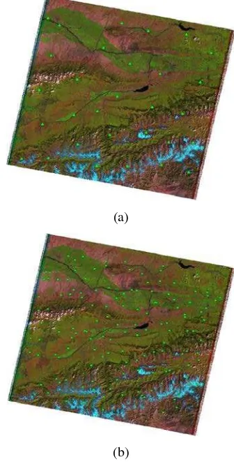
A scene of Landsat-5 TM L2 image (30 m) captured in July 2009 was used to perform the experiments. The image is in Aksu district, Xinjiang province of China, and the elevation range is from 600 m to 4000 m, including some high mountains. Another scene of Landsat-5 TM L4 image (ortho product) in the same place captured in August 2007 was used as the reference image. As the two images were both acquired by Landsat-5 TM sensor in the same season of different years, 169 tie points from the two images were collected by the automatic matching module of PCI Geomatics 2013 software, and 30 evenly distributed tie points were chosen as ground control points (GCPs) while the other 139 points were used as checkpoints. The image and distribution of GCPs and checkpoints are shown in fig. 1.
(a)
(b)
4.2 Geometric rectification and uncertainty estimation 4.2.1 Geometric rectification and accuracy report
The rigorous sensor model (Kramer, 2002) of Landsat-5 L2 was used to perform rectification with the help of GCPs and DEM data (ASTER GDEM Version 2), and then the residual of GCPs and checkpoints can be calculated to evaluate the accuracy of the rectified image. As shown in Table 1, the root mean square errors (RMSEs) and the maximum residuals of GCPs and checkpoints are included.
RMSE/pixel Max/pixel
x y x y
GCPs 0.564 0.146 -0.946 -0.48
checkpoints 0.733 0.161 2.617 -0.65
Table 1. Accuracy report of the geometric rectification.
From Table 1, one can see that the residuals of checkpoints are greater than those of GCPs. This is reasonable as the GCPs were utilized to estimate the geometric model while the checkpoints were not. Accordingly, the residuals of checkpoints are the most frequently used approach to objectively evaluate the geometric accuracy of rectified image. However, the residuals of checkpoints only show the accuracy of a few points in the image, and collecting a large number of checkpoints will be time- and labour-consuming.
4.2.2 Error and uncertainty evaluation
As described in Section 2.3, the GCPs can be used to calculate the coefficients of the error model (7). By applying L1LS method, sparse coefficients can be obtained as,
1
a
~a
8: (-175.69, -25.834, 0, 0, 13.418, 0, 0, -1.3799) 1b
~b
8: (22.555, 0, 0, 0, 0, 0, 0.30619, -0.0078451) 1c
~c
8: (0, -5.6858, 0, 0, 3.5439, 0, 0, 1.2259) 1d
~d
8: (4.8106, 0, 12.834, 0, 0, 0, -0.0019516, -0.22948)As the rigorous sensor model of Landsat-5 L2 includes 8 parameters, the number of the coefficients of the error model is 32. One can see that many of the coefficients (more than a half)
are zeros, which indicates that some of the coefficients are not significant or correlated with other coefficients. Then the estimated coefficients can be used to calculate the possible error of any point.
To evaluate the proposed error model, the possible errors of checkpoints are predicted, and by comparing the predicted errors with the actual residuals of the checkpoints, one can see how well the error model predicts the possible error of any point. Table 2 shows the root mean square errors and maximum errors of the predicted error of the 139 checkpoints.
RMSE/pixel Max/pixel
x y x y
Error of prediction 0.409 0.162 1.519 0.565
Table 2. The error of the prediction of the error model.
From Table 2, one can see that the predicted errors of the checkpoints are very close to the actual residuals. Furthermore, according to Table 1 and Table 2, both the RMSEs and maximum errors of the predicted error are smaller than those of the geometric model.
On the other hand, one can further calculate the uncertainty of any point, say at a confidence level of 95%, according to formula (11) and formula(13). Table 3 shows the residuals and uncertainties of 30 GCPs, while Table 4 shows the residuals, predicted errors and uncertainties of 139 checkpoints.
ID Position Residual Uncertainty
x y x y x y
1 879 756 0.248 -0.145 1.105 0.286 2 4117 5160 -0.632 -0.035 1.105 0.286 3 439 583 0.433 0.118 1.105 0.286 4 6267 4976 -0.246 0.287 1.105 0.286
…… …… …… …… …… …… ……
…… …… …… …… …… …… ……
28 4586 2975 0.26 0.157 1.105 0.286 29 5385 4070 0.68 -0.057 1.105 0.286 30 2724 3459 0.463 0.069 1.105 0.286
Table 3. The residuals and uncertainties of the GCPs (pixels).
ID Position Residual Predicted error Uncertainty
x y x y x y x y
1 5849 4590 1.683 0.358 0.164 0.015 0.352 0.525
2 2750 4662 -1.158 -0.65 -0.396 -0.085 0.281 0.27 3 6011 3921 -0.637 0.106 -0.134 -0.034 0.353 0.502 4 6149 4162 0.807 0.12 -0.041 -0.015 0.359 0.533
… … … …
… … … …
137 1858 3101 0.196 -0.01 0.287 0.026 0.25 0.236
138 5544 1833 0.83 0.062 0.424 0.1 0.331 0.36
139 4956 2151 1.016 0.117 0.713 0.127 0.313 0.325
Table 4. The residuals, predicted errors and uncertainties of the checkpoints (pixels).
As can be seen from the Table 3 and Table 4, representing data by form is not intuitive and not conducive to observation. Therefore, appropriate visualization of data is particularly important, and the following section will focus on the visual expression of the errors and uncertainties.
4.3 Visualization of error and uncertainty 4.3.1 Discrete representation
ID of point
0 5 10 15 20 25 30
E
rro
r
-1.2 -1.0 -.8 -.6 -.4 -.2 0.0 .2 .4 .6 .8 1.0
Error of x Error of y
Figure2. Errors of GCPs.
Figure3. The true errors and the predicted errors of CPs.
From fig. 3, we can see that the true error of CPs is larger than the predicted error in general. But visualization by histogram can only express the value of uncertainty. If the information of spatial distribution is needed, we can visualize the uncertainty by arrow vector, just as shown in fig. 4 and fig.5.
Figure 4. Visualizing the uncertainty of GCPs by arrow vector (the rectangles represent the uncertainty of GCPs)
Figure 5. Visualizing the uncertainty of CPs by arrow vector (the rectangles represent the uncertainty of CPs)
As can be seen from the Fig. 4 and 5, visualizing the uncertainty by arrow vector can not only express the direction, but also can express the value of uncertainty to some extent.
4.3.2 Continuous representation by interpolation
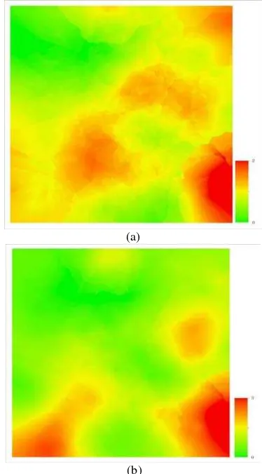
With the help of Kriging interpolation, we can also obtain the error of each point from the errors of checkpoints, and then visualize the error in surface or contours with the visual variable, as shown in fig. 6. Fig. 6(a) shows the possible errors predicted by the error model(7), and fig. 6(b) shows the actual errors (or residuals of checkpoints).
(a)
(b)
Figure 6. Visualizing the errors of CPs in remote image by iso-surface. (a) shows the predicted errors and (b) shows the actual
errors (residuals).
As can be seen from the fig. 6, the predicted error is consistent with the true error in general. This means the error model is credible.
(a)
(b)
(c)
Figure 7. Error absolute values of the pixels in the whole image and the corresponding DEM data. (a) shows the error absolute values in x direction while (b) shows those in y direction, and (c)
is the distribution of DEM value.
In this experiment the positional errors are mainly from the errors of GCPs, DEM, and geometric model. The errors from GCP are small since both the distribution (fig.1) and RMSEs (table 1) of the GCPs are good enough, and the error from the geometric model is omitted, so the main displacement is from DEM or the attitude difference. This can be seen from fig. 7 clearly. According to fig. 7, it can be observed that the distribution of error is quite related to the DEM data, but the relationship is not positive correlation or negative correlation. Actually, great errors are likely to be produced by both great and small elevation values, while the intermediate values of DEM may result in small geometric errors. Moreover, by comparing fig.7(a) and fig. 7(b) with fig. 6(b), one can see that the distribution of the predicted error is similar to the error map interpolated from the residuals of checkpoints.
Additionally, uncertainty of each point in the image can also be calculated by the uncertainty model described as formula (11) and formula(13), and fig. 8 shows the uncertainties of the pixels in the whole image.
(a)
(b)
Figure 8. Uncertainties of the pixels in the whole image. (a) shows the uncertainties in x direction, and (b) shows those in y
direction.
Different from the case of predicted errors, the distribution of predicted uncertainties is much smoother, and is not obviously related the DEM data. The uncertainties show the position quality where is much reliable and where is less.
Finally, both the predicted errors and predicted uncertainties as shown in fig. 7 and fig. 8 can be generated as auxiliary products of geometric rectified products to evaluate the geometric quality of the processed images.
5. CONCLUSIONS AND SUGGESTIONS
The work in this study can be concluded as several points. Firstly, a generic error model is proposed to evaluate the possible positional error of any point on the image based on the error propagation theory of indirect measurement. Secondly, an uncertainty model is deduced according to the propagation theory of uncertainty. Thirdly, several visualization methods are studied to represent the discrete and continuous data of geometric uncertainties.
which are benefit for the users to comprehend the data quality. Part of our future work is to test with more images and to further study the other error estimation models.
ACKNOWLEDGEMENTS
The research has been supported by the grant from the National Natural Science Foundation of China (61271013) and the Director Foundation of Institute of Remote Sensing and Digital Earth, CAS (Y5ZZ10101B).
REFERENCES
Arnoff S., 1985. The minimum accuracy value as index of classification accuracy. Photogrammetric Engineering &
Remote Sensing, 51(1): 593-600.
Bastin, L., Fisher,P. F., Wood J., 2002. Visualizing uncertainty in multi-spectral remotely sensed imagery. Computer &
Geosciences, 28(3), 337-350.
Bastin, L., Fisher, P.F. and Wood, J., 2002. Visualizing uncertainty in multi-spectral remotely sensed imagery, Computers & Geosciences, 28(3): 337-350.
Beard, M.K. and Mackaness, W., 1993. Visual access to data quality in geographic information systems. Cartographica, 30(2+3): 37-45.
Bevington, Philip R.; Robinson, D. Keith, (002. Data Reduction
and Error Analysis for the Physical Sciences (3rd ed.),
McGraw-Hill, ISBN 0-07-119926-8.
Blenkinsop, S., Fisher, P., Bastin, L., and Wood, J., 2000. Evaluating the perception of uncertainty in alternative visualization strategies. Cartographica, 37, 1–13.
Buiten, H. J. and Van Putten, B. , 1997. Quality assessment of remote sensing image registration and testing of control point residuals. ISPRS J. Photogramm.Remote Sens., 52(2), 57–73.
Ge Y., Liang Y., Ma J., Wang J., 2006. Error propagation model for registration of remote sensing image and simulation analysis.
Journal of Remote Sensing, 10(3), 299-305.
Goncalves, H., Goncalves, J. A., Cort-Real, L., 2009. Measures for an objective Evaluation of the geometric correction process quality. IEEE Geoscience and Remote Sensing Letters, 6(2), 292-296.
Janssen, L.L.F., Van Der Wel, F.J.M., 1994. Accuracy Assessment of Satellite Derived Land-Cover Data: A Review,
Photogrammetric Engineering & Remote Sensing, 60(4),
419-426.
Jiao W., Cheng B., Zhu W., Liu W., He G., Wang W., Zhang X., 2008. Accuracy Analysis of Remote Sensing Image Rectification, In Proc. SPIE - Remote Sensing of the Environment: 16th National Symposium on Remote Sensing of
China, Vol. 7123, 712308.
Kramer, O., 2002. Open Source Software Image Map (OSSIM) Project.http://trac.osgeo.org/ossim/browser/trunk/ossim/src/ossi m/projection/ossimLandSatModel.cpp (10 July 2015).
Lei H, Chen H, Xu J, Wu X, Chen W, 2013. A Survey on Uncertainty Visualization. Journal of Computer-Aided Design
& Computer Graphics, 25(3), 294-303.
Long, T., Jiao, W., He, G., Zhang, Z., Cheng, B., Wang, W. , 2015. A Generic Framework for Image Rectification Using Multiple Types of Feature, In ISPRS Journal of
Photogrammetry and Remote Sensing, 102(4), 161–171.
Long, T., Jiao, W., He, G., 2015. RPC Estimation via L1-Norm-Regularized Least Squares (L1LS). IEEE Transactions on
Geoscience and Remote Sensing, 53 (8), 4554–4567.
Lucieer A. And Kraak, M., 2004. Interactive and visual fuzzy classification of remotely sensed imagery for exploration of uncertainty, Int. J. Geographical Information Science, 18(5), 491–512.
MacEachren, A.M., Taylor, D.R.F. (Eds.), 1994. Visualization
in Modern Cartography, Pergamon Press, Oxford.
Van Der Wel, F.J.M., Hootsmans, R.M., Ormeling, F., 1994. Visualization of data quality, In McEachren, A.M.,
Taylor,D.R.F. (Eds.), Visualization in Modern Cartography.
Pergamon Press, Oxford, 313-331.
Van Der Wel, F., Van Der Gaag, L., and Gorte, B., 1997. Visual exploration of uncertainty in remote sensing classification.
Computers & Geosciences, 24, 335–343.