A first-order closure model for the wind flow within
and above vegetation canopies
Pingtong Zeng
∗, Hidenori Takahashi
Laboratory of Geoecology, Graduate School of Environmental Earth Science, Hokkaido University, Sapporo 060-0810, Japan Received 18 March 1999; accepted 11 January 2000
Abstract
A first-order closure model that has the general utility for predicting the wind flow within and above vegetation canopies is presented. Parameterization schemes that took into account the influence of large turbulent eddies were developed for the Reynolds stress and the mixing length in the model. The results predicted by the model were compared with measured data for wind speeds within and above six types of vegetation canopy, including agricultural crops, deciduous and coniferous forests, and a rubber tree plantation during fully leafed, partially leafed and leafless periods. The predicted results agreed well with the measured data; the root-mean-square errors in the predicted wind speeds (non-dimensionalized by the friction velocity above the canopy) were about 0.2 or less for all of the canopies. The secondary wind maxima that occurred in the lower canopies were also correctly predicted. The influence of foliage density on the wind profiles within and above a vegetation canopy was successfully simulated by the model for a rubber tree plantation during fully leafed, partially leafed and leafless periods. The bulk momentum transfer coefficients (CM) and the values ofλ(which are defined by z0=λ(h−d), where z0
is the roughness and d is the zero-displacement height of the canopy) for the vegetation canopies were also studied, and the relationships CMh=0.0618 exp(0.792CF) andλ=0.209 exp(0.414CF) were determined; here, CMhis the bulk momentum
transfer coefficient at the canopy top; CF=CdPAI zmax/h, where Cdis the effective drag coefficient of the canopy, PAI is the
plant area index and zmaxis the height at which the plant area density is maximum. The values ofλranged from 0.22 to 0.32
for the canopies studied. © 2000 Elsevier Science B.V. All rights reserved.
Keywords: Numerical model; Wind velocity; Vegetation canopy; Reynolds stress; Mixing length; Turbulent eddy
1. Introduction
Wind is an important factor for scalar fluxes (heat, water vapor, carbon dioxide, etc.) and movements of spores, pollen and particles within a vegetation canopy. Information about the wind flow within the vegeta-tion canopy is important in meteorological, agricul-tural and ecological studies. A number of numerical models for predicting the vegetation wind flow have
∗Corresponding author. Fax:+81-11-706-4867.
E-mail address: [email protected] (P. Zeng)
been developed. However, accurate prediction of wind flow is difficult due to the complexity in the array of vegetation elements (leaves, branches and so on) and the complex process of air momentum transport within a vegetation canopy. Early modeling studies (e.g. In-oue, 1963; Cowan, 1968; Thom, 1971) were based on the K-theory or gradient-diffusion theory; that is, the momentum flux is equal to the product of an eddy viscosity and the local gradient of mean wind ve-locity. Wilson and Shaw (1977) (hereafter WS) point out that a K-theory model provides little insight into the nature of momentum transport processes within
the vegetation canopy. Moreover, Pereira and Shaw (1980) and Watanabe and Kondo (1990) (hereafter WK) show that such a model can not provide accurate predictions of wind velocity in the lower portion of a plant canopy, where a near-zero vertical gradient of mean wind velocity or a wind velocity ‘bulge’ is fre-quently observed (Shaw, 1977). In another approach, WS proposed a higher-order (second-order) closure model in which turbulent kinetic energy equations and Reynolds stress equation were solved simultaneously with that for mean momentum. However, WS reported that the calculated velocity profile was sensitive to the parameterization scheme for the turbulent transport term in their model. In order to avoid the deficiency in the model of WS, Meyers and Paw (1986) (here-after MP) developed a third-order closure model using third-order closure principles. However, the utility of a higher-order closure model is still limited. The model proposed by MP includes about 10 equations for only a one-dimensional problem, and the computation cost is therefore high. In addition, their modeled results for the turbulent field have large errors (MP; Meyers and Baldocchi, 1991). The parameterization schemes for higher-order closure models used for predicting veg-etation wind flow need to be further improved (MP; Shaw and Seginer, 1987; Wilson, 1988).
As an alternative approach that does not use higher-order closure principles, Li et al. (1985) pro-posed a non-local closure scheme for the total mo-mentum flux (Reynolds stress and dispersive flux) and developed a first-order closure model that was capable of predicting the wind velocity peaks in lower canopies. However, several problems in their model have been pointed out by Van Pul and Van Boxel (1990). To correct these problems, Miller et al. (1991) (hereafter MLL) made some modifications to their model and applied it to wind flow across an alpine forest clearing. However, the utility of their model for different types of vegetation canopy was not tested. Over the past few decades, extensive measurements (e.g. Raupach et al., 1986; Shaw et al., 1988; Gao et al., 1989) of turbulent flows within and above vege-tation canopies have been carried out. On the basis of the results of the previous studies, the purpose of the present study is to develop a first-order closure model, which is simple in computation and has the general utility for predicting wind flow within and above vegetation canopies, and to investigate the
in-fluences of canopy structure and foliage density on the wind velocities within and above the canopies.
2. Theory and the model
2.1. Governing equation
Following Raupach et al. (1986), under neutrally buoyant conditions, the time- and volume-averaged equation for the mean momentum within vegetation is
∂huii
Here, i and j are index notations (with values of 1–3) and Einstein’s summation is used. The overbars and single primes denote time averages and fluctuations, while the angle brackets and double primes denote spatial volume averages and departures therefrom, re-spectively. ui and xi are velocity and position
vec-tors, respectively, t the time, p the kinematic pressure,
fFi andfVi are form and viscous drag force vectors exerted on a unit mass of air within the averaging volume, respectively,τij the volume-averaged
kine-matic momentum flux or stress tensor, and ν is the kinematic viscosity. Interpretations of each term in the above equations have been described by Raupach et al. (1986).
For a horizontal homogeneous vegetation, let u and
fx(=fF1+fV1) is the total streamwise drag per unit
mass of air within the averaging volume. These terms must be parameterized in order to solve the equation and estimate the wind velocityhui.
2.2. Closure schemes
2.2.1. Reynolds stress
In K-theory models, the Reynolds stress is param-eterized as
hu′w′i = −KM
dhui
dz (4)
where KMis the eddy viscosity. This model shows that
the turbulent flux of momentum results from the local gradient in the mean wind velocity. Hence, it is also called a small-eddy closure technique (Stull, 1988). K-theory models have been widely used for studies in the surface layer and have been proven to be reli-able for the inertial sublayer above a surface (Raupach et al., 1980). However, Corrsin (1974) has pointed out that the application of K-theory is limited to the place where the length scales of flux-carrying motions have to be much smaller than the scales associated with average gradients. It is unfortunate that such a condi-tion is often violated within vegetacondi-tion canopies (Rau-pach and Thom, 1981; Baldocchi and Meyers, 1988b). Many measurements have shown that wind flow within and just above a plant canopy is dominated by turbu-lence with vertical length scales at least as large as the vegetation height (Kaimal and Finnigan, 1994). These large-scale turbulent eddies are intermittent and ener-getic, and they can penetrate the canopy crowns and enter the subcanopy trunk space to generate non-local turbulent transport. Most of the transport of momen-tum and scalar properties within the canopy are gen-erated by these large-scale turbulent eddies (Raupach et al., 1986; Baldocchi and Meyers, 1988a). Baldoc-chi and Meyers (1988b) report that the Reynolds stress within a plant canopy is influenced not only by the product of KM and the local vertical gradient in the
mean wind velocity but also by the non-local turbulent transport through the activities of large-scale eddies.
Based on the results obtained from previous studies, the turbulent momentum flux is divided into two parts in the present study: one diffused by the smaller-scale eddies, which depends on the local gradient of the mean wind velocity; and the other transported by the
larger-scale eddies, which is determined by the mean wind speed differences between heights with large dis-tance. Hence, the Reynolds stress is parameterized by
−hu′w′i =Kdhui
dz +Cghuri(huri − hui) z
h (5)
where K is the eddy viscosity, h the vegetation height,
ur the wind velocity at a reference height above the
vegetation, and Cgis a coefficient. On the right-hand
side of the equation, the first term (defined as Rs),
which has been formed according to the conventional K-theory, is responsible for small-eddy diffusion, and the second term (defined as Rl) is responsible
for non-local transport. Since non-local transport is caused by the shear between the wind flows above and within the canopy, we usedhuri − huito represent the
intensity of the shear.hurioutside of the parentheses
was used to account for the intensity of the wind flow above the canopy. As it is easier for turbulent eddies to penetrate into a sparse canopy than into a dense canopy (Shaw et al., 1988), the coefficient Cgin the
equation is defined to be a function of the integrated plant area density and is expressed by
Cg=C1exp
fective drag coefficient of the plant elements, and C1
and C2are constants that are determined by numerical
experiments. The second term in Eq. (5) is an addi-tional term that we have introduced. This term is sim-ilar to the term that represents dispersive flux in the model proposed by MLL, but instead of Cgdefined in
and negligible compared with the amount of turbu-lent flux. In addition, wind velocities within vegetation canopies have been successfully predicted by WS and MP, who used higher-order closure models in which a term of dispersive flux is not included. Therefore, dispersive flux is considered to be negligible and was omitted in the present study.
2.2.2. Mixing length
The eddy viscosity K is parameterized according to the Prandtl–von Kármán mixing-length theory
K=l2
where l is the mixing length. Above the vegetation canopy surface, the mixing length is expressed as
l=κ(z−d), z≥h (8)
whereκ is the von Kármán’s constant equal to 0.4, and d is the zero-plane displacement (m). The mix-ing length within a canopy is complicated due to the effects of canopy elements. In conventional K-theory models, Inoue (1963) suggested that l is constant throughout the canopy layer, while Seginer (1974), Kondo and Akashi (1976) and WK considered l to be constrained by the ground surface and the local internal structure of the canopy and defined it as a function of the local plant area density, drag coeffi-cient and height. As the conventional K-theory model is used in the present model to represent only the small-eddy diffusion within the canopy, the definition of mixing length within the canopy in the present model is different from that in conventional K-theory models. However, the effects of ground surface and canopy structure pointed out by Seginer (1974) and other researchers will be qualitatively the same. In addition, it is considered that the value of l within the canopy can not be larger than that at the canopy top lh (= κ(h−d) according to Eq. (8)). Thus, the
mixing length within the canopy is parameterized as
l= κz
1+ClCdAz
(9)
with
l≤(h−d), z < h
where Cl is a constant determined by numerical
ex-periments. This model is different from that proposed
by MLL, which is a function of z and the total leaf area in the portion below d and does not reflect the effect of local canopy structure.
2.2.3. Drag force
The drag of plant elements fx is parameterized
ac-cording to WS
fx=CdAhui2 (10)
This parameterization scheme has been widely used in studies on wind flow within a vegetation canopy (e.g. MP; WK; Wang and Takle, 1996). The effective drag coefficient (Cd) of a single leaf measured in wind
tunnel changes with the leaf orientation and turbu-lent scales and intensity around the leaf (Raupach and Thom, 1981). However, MP reported that the value of
Cd of a vegetation canopy is a constant, i.e. it does
not depend on wind speed and the position within the canopy.
3. Numerical aspects
The selected reference height for the reference wind speedhuri is twice the vegetation height. This
selec-tion is based on measurements showing that there is a roughness sublayer within which the eddy viscos-ity is found to be enhanced and the semi-logarithmic law is not obeyed over a rough surface (e.g. Garrat, 1978; Raupach et al., 1980; Simpson et al., 1998). Three new parameters are introduced in the present model: C1and C2 in Eq. (6) and Cl in Eq. (9). The
values of these three parameters were firstly fitted to be 0.01, 1.0 and 5.0, respectively, by using the corn canopy data, but C2was adjusted to 2.0 in the
simula-tions for the rubber canopy data. Variasimula-tions in C2only
affect the modeled wind profile at the lower canopy. The final values of 0.01, 2.0 and 5.0 for C1, C2 and Cl, respectively, were used for all the canopies in the
present study. The computation grid included 60 equal intervals from the ground surface to three times the vegetation height. All variables in the model were non-dimensionalized by scales of h and the wind speed at 3h height. Non-dimensional wind speed was given by 1 at the upper boundary and 0 at zg/h=0.001, where zg is the roughness length of the ground surface.
sensitive to the chosen of the value zg. The initial wind
profile was assumed, and the solution was found iter-atively until the differences in the computedhuiwere less than the control level (10−4in this study).
4. Results and discussion
4.1. Wind profiles in various types of vegetation canopy
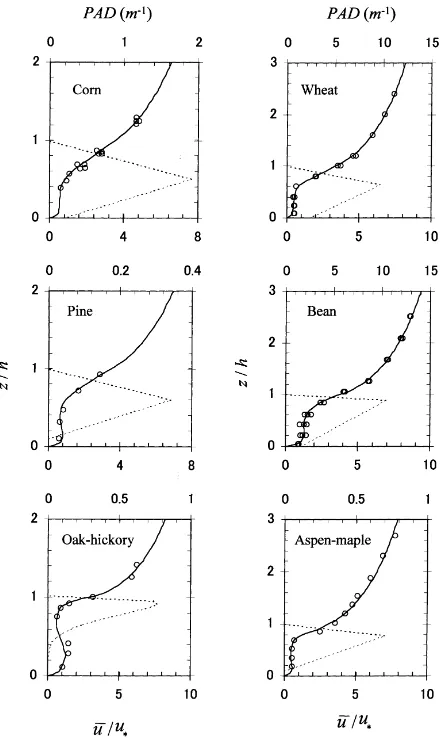
Wind speeds were predicted by the present model within and above six types of vegetation canopy, which included agricultural crops, and deciduous and conif-erous forests with leaf area indices (LAI) from about two to near seven and vegetation heights from about 1 m to more than 20 m (Table 1). The predicted and measured wind-speed profiles ranging from ground surface to twice the canopy height for three canopies and to three times the canopy height for the other three canopies, are shown together with the distributions of plant area density (PAD) in Fig. 1. The measured wind profiles in the pine and oak–hickory forests were av-erages. The leaf area density of the pine forest was the average of pine A and pine B in Amiro (1990a), and the tree height of 18.5 m was used in the present study, which was based on the reported tree height of 15–20 m for the pine forest. Though the measured wind profiles within and above the canopies show large differences according to the species and structure of the canopies, the predicted wind profiles matched them excellently. The measured wind profiles in most of the canopies show small gradients or slight reversals
Table 1
List of vegetation canopies and the references. Oak–hickory and aspen–maple are mixed deciduous forests with principal species of oak and hickory, and aspen and maple, respectivelya Vegetation h (m) LAI References canopies
Corn 2.8 3 Wilson and Shaw (1977) Pine 18.5 2.3 Amiro (1990a)
Oak–hickory 23 4.9 Meyers and Baldocchi (1991) Bean 1.18 6.3 Thom (1971)
Wheat 1.25 6.6 Legg (1975a, b) Aspen–maple 18 5 Neumann et al., (1989);
Gao et al. (1989)
ah is the vegetation height, and LAI is the leaf area index.
Fig. 1. Comparison of predicted (solid lines) and measured (circles) wind speeds within and above six types of vegetation canopy. Vertical distributions of plant area density (PAD, dashed lines) are also shown. Wind profiles ranging to 2h (h is vegetation height) are shown for corn, pine and oak–hickory canopies, and those ranging to 3h are shown for wheat, bean and aspen–maple canopies. u∗is
the friction velocity above the canopy.
in gradient in the lower portion of the canopies, and an obvious secondary maximum can be seen in the oak–hickory canopy. K-theory models are incapable of predicting these features. The present model suc-cessfully demonstrated these features, revealing that the non-local transport was accurately considered in the model. It was revealed by the present model that though the small-eddy diffusion Rs was near zero or
gradient of mean wind was reversed, the non-local transport Rl was large and maintained the Reynolds
stress in the lower canopies (see also Section 4.4). Shaw (1977) has pointed out that the mean wind gra-dient will be reversed if the non-local turbulent trans-port momentum is large enough in the lower trans-portion of a vegetation canopy, i.e.
∂w′u′w′
He also suggested that in the region where there is a re-versal in mean wind gradient, larger scales of turbulent motion transport momentum downward, while smaller scales transport momentum upward according to the local gradient. Very strong wind shear appears near the canopy top in two deciduous canopies (oak–hickory and aspen–maple canopies) because there are very dense foliage layers at the upper portion of these two canopies. The foliage is also very dense at the upper portion of the bean canopy, but the wind shear is not as large as that in the deciduous canopies, because the drag coefficient of the bean canopy is very small (Table 3). The wind speed within the wheat canopy, which has the greatest foliage density, is very low. The predicted wind profile within the pine canopy is also very similar to those measured in other pine forests that have similar distributions of foliage densities (e.g. Allen, 1968; Halldin and Lindroth, 1986).
Shaw and Pereira (1982) reported that the wind pro-file predicted by their second-order closure model was not logarithmic immediately above the canopy sur-face. However, many researchers have observed loga-rithmic or near-logaloga-rithmic wind profiles above many vegetation canopies (e.g. Thom, 1971; Oliver, 1971; Dolman, 1986). Fig. 1 shows that the predicted and measured wind profiles above the bean canopy are al-most the same. The measured profiles were the profiles of D–F in Fig. 7 of the report by Thom (1971), which were reported to be logarithmic above the canopy. The wind profile above a canopy computed by the present model is approximately logarithmic because the non-local transfer (Rl) is small above a canopy (see
also Section 4.4). The roughness sublayer over a plant canopy is believed to be shallow (e.g. Simpson et al., 1998) except in cases where the canopy is very sparse (e.g. Garrat, 1978). In order to predict the wind profile above the canopy, a correct value for the zero-plane
Table 2
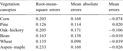
Mean errors in predicted wind speeds (non-dimensionalized by the friction velocity above the canopy)
Vegetation Root-mean- Mean absolute Mean canopies square errors errors errors
Corn 0.203 0.168 −0.074
Pine 0.126 0.114 0.020
Oak–hickory 0.205 0.171 −0.106
Bean 0.163 0.138 −0.010
Wheat 0.135 0.098 −0.039
Aspen–maple 0.233 0.168 −0.026
displacement (d) is needed. This value is estimated by the model based on an additional input value of mea-sured wind speed above the canopy. Experimental re-sults showed that the predicted wind profile within the canopy was not sensitive to the choice value of d if d is lower than 0.85 h.
Predicted results according to higher-closure mod-els (e.g. MP; Shaw and Seginer, 1987; Meyers and Baldocchi, 1991) often show larger errors near the canopy top, where strong shear in the flow field occurs. The present model does not have this prob-lem. Table 2 shows the mean, mean absolute and root-mean-square errors in predicted results calcu-lated by comparing predicted and measured values. The largest root-mean-square error is 0.23 (for the oak–hickory canopy), and other root-mean-square errors are 0.2 or less. The mean absolute errors are smaller than 0.2, and the mean errors are almost zero for all canopies. MP compared their predicted results by using a higher-order closure model with measured data for six canopies (in which corn and bean canopies were the same as those used in the present study). Their root-mean-square errors were larger than 0.2 for most canopies, and the largest error was 0.54; these values were larger than those in the present study.
Table 3
Comparison of drag coefficients (Cd) yielded by the present model and those estimated in other studies
Vegetation Present Other References canopies study studies
Corn 0.20 0.20 Wilson and Shaw (1977) Pine 0.20 0.1–0.25 Amiro (1990b) Oak–hickory 0.18 0.15 Lee et al. (1994) Bean 0.04 0.03–0.04 Thom (1971)
between the modeled results and the measured data in the present study suggests that this technique is use-ful for numerical studies of wind flow within vege-tation canopies. A beta distribution, which was used by Meyers and Baldocchi (1991), was used for the aspen–maple canopy in the present study.
As was the case in the study by MP, a constant effective drag coefficient (Cd) for each canopy was
used in the present study. The effective drag coeffi-cient for a vegetation canopy is difficult to measure due to problems of the shelter effect (Thom, 1971) and leaf orientation. In numerical studies, it is usually de-termined by trial-and-error to produce the best agree-ment with observations. The effective drag coefficient for each canopy in the present study was determined by trial-and-error. Table 3 shows a comparison of the values of Cd yielded by the present model and those
estimated in other studies for the same canopies. It is shown that those yielded by the present model are almost the same as or within the range of those es-timated in other studies. The values of Cd used for
the wheat and aspen–maple canopies were 0.12 and
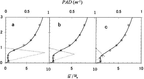
Fig. 2. Simulated (solid lines) and measured (circles) wind profiles in the rubber tree plantation during (a) fully leafed, (b) partially leafed and (c) leafless periods. Profiles of PAD are shown by dashed lines.
0.15, respectively; published values of Cd for these
two canopies are not available for comparison. The re-sults of the present study also support the claim made by MP that the use of a constant effective drag coef-ficient is appropriate for a plant canopy.
4.2. Influence of foliage density on the wind profile
Influence of foliage density on the wind profile was investigated using the data measured in a rubber plan-tation located in the Hainan Island, China. The rub-ber trees were about 12 m in height and the foliage density were estimated from the leaf-fall collections and the measured solar radiations. Detailed informa-tion of the instrumentainforma-tion and site has been described by Takahashi et al. (1986) and Yoshino et al. (1988). Fig. 2 shows the simulated (using the present model) and measured wind profiles in the rubber tree plan-tation during fully leafed, partially leafed and leaf-less periods. The measured profiles were averages in near-neutral conditions and when the wind direction was ESE, in which the effect of the surrounding wind-breaks was smallest and the fetch was the longest. The plant area indices (PAIs) during the three periods were about 5, 3 and 1, respectively.
of the rubber trees during the three periods. How-ever, the normalized wind speed (u/u∗) within the canopy increases as the foliage density decreases, because it is easier for momentum to penetrate the canopy from above the canopy if the canopy is thin. Although the PAI decreased about five-fold from the fully leafed to leafless periods, the normalized wind speed within the leafless canopy, except that at the very upper portion of the canopy, increased less than two-fold. This discrepancy can be explained by the effect of the effective drag coefficient. Seginer et al. (1976) has shown, from the results of wind-tunnel experiments, that the effective drag coefficient of a dense canopy is smaller than that of a thin canopy. The effective drag coefficients used by the model for the fully leafed and leafless canopies were 0.15 and 0.36, respectively, showing that the effective drag co-efficient of tree branches in a fully leafed canopy is smaller than that in a leafless canopy. The same fact was also found by Sato (personal communication) in his studies on wind flow through windbreaks. Each of the three wind profiles showed a weak secondary wind maximum in the lower portion of the canopy because the trunk space of the rubber plantation was very open. The wind profiles are near logarithmic above the three canopies, and the slope of the wind profile during fully leafed period is larger than that during leafless period. These findings are consistent with those observed above a Japanese larch forest (Allen, 1968) and an oak forest (Dolman, 1986).
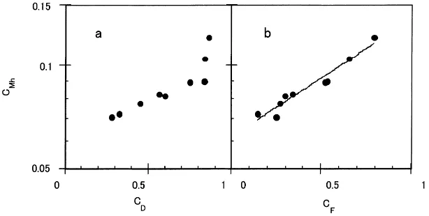
Fig. 3. Variation in the bulk momentum transfer coefficients at the canopy top (CMh) vs. (a) CD (=CdPAI) and (b) CF(=CdPAI zmax/h) for nine vegetation canopies.
4.3. Bulk momentum transfer coefficients
It can be seen in Figs. 1 and 2 that values of the normalized velocitiesu/u∗(u∗is the friction velocity above the canopy) at the top of all the canopy tops are very similar, but changes of them according to the type of canopy are discernible. The same phenomenon was also shown by MP. If the normalized velocity above the canopy is inverted and squared, it becomes the bulk momentum transfer coefficient CM, which is defined
as
τ ρ =u
2
∗=CMu2 (11)
whereτis the shear stress,ρthe air density, u∗the fric-tion velocity, anduis the mean wind speed at a height above the vegetation. CM is also called drag
coeffi-cient by some researchers. Dolman (1986) showed that
CM above an oak forest was about two-times larger
on foliated conditions than that on defoliated condi-tions. On the other hand, WK showed that CMover a
rice canopy was scattered in a wide range over peri-ods with differing leaf area indices. It is probable that the variations in the CMabove a vegetation canopy do
not depend only on the foliage density of the canopy. Fig. 3a shows the variations in the CM at the canopy
top versus CdPAI, where PAI is the plant area index,
there is a clear tendency for CMto increase as CdPAI
increases. Furthermore, when the variations in CMare
plotted against CdPAI zmax/h, where zmaxis the height
at which the plant area density is maximum, a good correlation between them is revealed (Fig. 3b). Shaw and Pereira (1982) have shown that zmaxis an
impor-tant factor in determining the aerodynamic roughness of a plant canopy. The value of CdPAI zmax/h is
small-est (0.146) in the case of the leafless rubber planta-tion canopy. It seems that CdPAI zmax/h can accurately
represent the momentum absorption ability of a vege-tation canopy. Let
CD≡CdPAI, (12)
CF ≡CD zmax
h (13)
and CMhrepresent the bulk momentum transfer
coef-ficient at the canopy top, then the fitting-curve for the nine canopies in Fig. 3b is expressed as
CMh=0.0618 exp(0.792CF) (14)
and the correlation coefficient was equal to 0.889. Us-ing a K-theory model, WK predicted that CMincreased
with an increase in CDwhen CD<0.3, but it decreased
with an increase in CDwhen CDincreased further for
a rice canopy. However, their prediction was not sup-ported well by the measured data.
If the logarithmic law is obeyed above a canopy surface, the wind profile above the canopy surface is expressed as
where z0is the roughness of the canopy surface. Thom
(1971) suggested that
z0=λ(h−d) (16)
where h is the canopy height, and the value ofλwas estimated to be 0.36 for an artificial crop. Seginer (1974) estimated the value ofλto be 0.37 on the basis of the canopy wind model of Inoue (1963) and an ob-servation by Kondo (1971). However, the value of λ
was estimated by Moore (1974) to be 0.26 according to 105 published d, z0and h data, and it was also
es-timated by Shaw and Pereira (1982) to be 0.26 (when
CD>0.2) on the basis of results of numerical
experi-ments using a higher-order closure model. From Eq. (15), we can get
z0=
1 exp(κ(uh/u∗))
(h−d) (17)
whereuhis the mean wind speed at the canopy top.
From Eqs. (11), (16) and (17) we find that
(according to Eq. (14)), and is not a constant when
CF>0.2. It was difficult to obtain a simple expression
for the relationship betweenλand CF from Eqs. (14)
and (18). However, the results of least-squares analysis for the values ofλand CFfor the nine canopies showed
that
λ=0.209 exp(0.414CF) (19)
with the correlation coefficient equaling 0.892. The values ofλfor the nine canopies ranged from 0.22 (the bean canopy) to 0.32 (the oak–hickory canopy), and the average for all of the canopies was 0.26, which is the same value as that obtained by Moore (1974) and Shaw and Pereira (1982). For comparison, Bruin and Moore (1985) reportedλ=0.22 for a pine forest (the Thetford Forest).
4.4. Reynolds stress
The computed Reynolds stress for the corn canopy showed that more than 80% of the momentum was ab-sorbed in the upper half of the canopy (Fig. 4), which was the same as that shown by the measured data. The computed Reynolds stress decreased to almost zero near the ground. Though there was no measured data for comparison in the lower canopy, the modeled re-sults were almost the same as those showed by WS, who computed using a higher-order closure model.
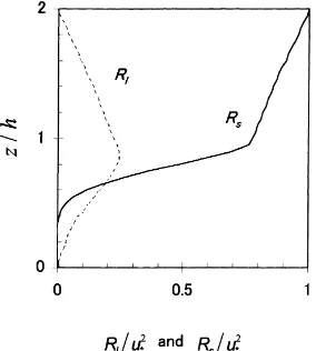
Fig. 5 shows the computed profiles of two com-ponents of the Reynolds stress, Rl and Rs, for the
corn canopy. Though Rs is larger than Rl above the
Fig. 4. Profile of the computed Reynolds stress (line) and the measured data (closed circles) for the corn canopy.
Rl. Meyers and Baldocchi (1991) have pointed out
that the shear production, which is generated by the interaction between the turbulent field and the mean velocity gradient, is small and turbulence imported from above the canopy is a strong source for the turbulent kinetic energy in the lower canopy. Thus, the present model can account for the phenomena of counter-gradient momentum transport and secondary wind maxima that occurs in the lower portions of veg-etation canopies. Rlpeaks at about 0.8h and decreases
above and below this height, and this distribution pattern is similar to those of the measuredhw′u′w′i
Fig. 5. Profiles of two components of the Reynolds stress in the corn canopy: small-eddy diffusion Rs (solid line) and non-local transfer Rl (dash line).
(non-local transport of the Reynolds stress) in many canopies (e.g. Shaw and Seginer, 1987; Baldocchi and Meyers, 1988a, b; Amiro, 1990a). Above the canopy,
Rs is more than three times larger than Rl and is the
main source of the Reynolds stress, implying that the predicted mean wind profile above the canopy is ap-proximately logarithmic. For the layer above 2h, the non-local transfer momentum is parameterized to be zero in the model. Though only the profiles for the corn canopy are shown, those for the other canopies are qualitatively the same.
5. Conclusions
Taking into account the non-local turbulent trans-port, we have developed a first-order closure model for predicting the wind flow within and above vege-tation canopies. The high accuracy and the universal utility of the model were verified by comparisons of modeled results and measured data in six types of vegetation canopy and a rubber tree plantation dur-ing fully leafed, partially leafed and leafless periods. The root-mean-square errors in the predicted wind speeds were about 0.2 or less for all of the canopies; these errors are smaller than those results from a higher-order closure model. The wind speeds in the lower canopies, which appeared to be almost constant or reversed in gradient, were also correctly predicted. In addition to its high accuracy and universal utility, the present model costs little computation time due to its simplicity. The model would be very useful for the applications for predicting vegetation wind flows or scalar fluxes (e.g. heat and water vapor) between the atmosphere and vegetated surfaces when it is coupled with other models.
Based on the modeled wind speeds using the present model, we were able to clarify the effects of canopy density, structure and effective drag coefficient on the bulk momentum transfer coefficient and the coefficient
λ, and we were also able to determine the correlations between CM and CFand betweenλand CF.
The Reynolds stress in the present model was parameterized by two terms: one representing the small-eddy diffusion, and one representing non-local transport through large-scale turbulent eddies. The modeled results showed that the non-local transfer component was small above the canopy but large, and the main source of the Reynolds stress, in the lower portion of the canopy. The model can also account for counter-gradient momentum transport occurs in the lower portion of a vegetation canopy. A parameteri-zation scheme was developed for the mixing length within a canopy.
6. Nomenclature
A plant area density (m2m−3)
C1, C2, Cl constants equal to 0.01, 2 and 5,
respectively
CD a coefficient equal to CdPAI Cd canopy effective drag coefficient CF a coefficient defined as CdPAI zmax/h Cg coefficient of non-local momentum
transport
CM bulk momentum transfer coefficient CMh bulk momentum transfer coefficient at
the canopy top
d zero plane displacement height (m)
fx total (form and viscous) streamwise drag
force (N)
fF form drag force (N) fV viscous drag force (N) h mean vegetation height (m)
i, j index notations, with values of 1, 2 or 3
K momentum eddy viscosity (defined in present study) (m2s−1)
KM conventional momentum eddy viscosity
(m2s−1)
l mixing length (m) LAI leaf area index (m2m−2)
lh mixing-length at vegetation canopy
top (m)
p kinematic pressure (Pa) PAD plant area density (m2m−3) PAI plant area index (m2m−2)
Rl non-local momentum transport (m2s−2) Rs small-eddy diffusion (m2s−2)
t time (s)
T time average interval (s)
u streamwise velocity (m s−1)
ui wind velocity vector (m s−1) ur wind velocity at a reference height
(m s−1)
u∗ friction velocity above vegetation canopy (m s−1)
hu′w′i Reynolds stress (m2s−2)
V volume (m3)
w vertical velocity (m s−1)
xi position vector (m)
z height (m)
z0 roughness of vegetation surface (m) zmax the height at which the plant area
density is maximum (m)
Greek letters
ν kinematic viscosity of the air (m2s−1)
κ von Karm´ an’s constant (equal to 0.4)´
λ the coefficient between z0andλ ρ air density (kg m−3)
τ shear stress (m2s−2)
τij kinematic momentum flux (m2s−2) φ a scalar or vector variable
Other symbols
overbar ( – ) time average
prime (′) deviation from time average angle bracketsh i volume average
double prime (′′) deviation from volume average
Acknowledgements
Nos. 61041012 and 62043011). We are grateful to Prof. T. Maitani (Okayama University), Mr. T. Sato (Hokkaido Head Office, Japan Weather Association) and Mr. Natsume (Hokkaido Institute of Environmen-tal Science) for their helpful comments. Mr. Natsume also checked our computing programs.
References
Allen, L.H. Jr., 1968. Turbulence and wind speed spectra within a Japanese larch plantation. J. Appl. Meteorol. 7, 73–78. Amiro, B.D., 1990a. Comparison of turbulence statistics within
three boreal forest canopies. Boundary-Layer Meteorol. 51, 99–120.
Amiro, B.D., 1990b. Drag coefficients and turbulence spectra within three boreal forest canopies. Boundary-Layer Meteorol. 52, 227–246.
Baldocchi, D.D., Meyers, T.P., 1988a. Turbulence structure in a deciduous forest. Boundary-Layer Meteorol. 43, 345–364. Baldocchi, D.D., Meyers, T.P., 1988b. A spectral and
lag-correlation analysis of turbulence in a deciduous forest canopy. Boundary-Layer Meteorol. 45, 31–58.
Bruin, H.A.R., Moore, C.J., 1985. Zero-plane displacement and roughness length for tall vegetation, derived from a simple mass conservation hypothesis. Boundary-Layer Meteorol. 31, 39–49. Corrsin, S., 1974. Limitations of gradient transport model in random walks and in turbulence. Adv. Geophys. 18A, 25–60. Cowan, I.R., 1968. Mass, heat and momentum exchange between
stands of plants and their atmospheric environment. Quart. J. R. Meteorol. Soc. 94, 523–544.
Dolman, A.J., 1986. Estimates of roughness length and zero plane displacement for a foliated and non-foliated oak canopy. Agric. For. Meteorol. 36, 241–248.
Gao, W., Shaw, R.H., Paw, U.K.T., 1989. Observation of organized structure in turbulent flow within and above a forest canopy. Boundary-Layer Meteorol. 47, 349–377.
Garrat, J.R., 1978. Flux-profile relations above tall vegetation. Quart. J. R. Meteorol. Soc. 104, 199–211.
Halldin, S., Lindroth, A., 1986. Pine forest microclimate simulation using different diffusivities. Boundary-Layer Meteorol. 35, 103–123.
Inoue, E., 1963. On the turbulent structure of air flow within crop canopies. J. Meteorol. Soc. Jpn. 41, 317–325.
Kaimal, J.C., Finnigan, J.J., 1994. Atmospheric Boundary Layer Flows: Their Structure and Measurement. Oxford University Press, New York, p. 289.
Kondo, J., 1971. Relationship between the roughness coefficient and other aerodynamic parameters. J. Meteorol. Soc. Jpn. 49, 121–124.
Kondo, J., Akashi, S., 1976. Numerical studies on the two-dimensional flow in horizontally homogeneous canopy layers. Boundary-Layer Meteorol. 10, 255–272.
Lee, X., Shaw, R.H., Black, T.A., 1994. Modelling the effect of mean pressure gradient on the mean flow within forests. Agric. For. Meteorol. 68, 201–212.
Legg, B.J., 1975a. Turbulent diffusion within a wheat canopy: I. Measurement using nitrous oxide. Quart. J. R. Meteorol. Soc. 101, 591–610.
Legg, B.J., 1975b. Turbulent diffusion within a wheat canopy: II. Results and interpretation. Quart. J. R. Meteorol. Soc. 101, 611–628.
Li, Z.J., Miller, R., Lin, J.D., 1985. A first-order closure scheme to describe counter-gradient momentum transport in plant canopies. Boundary-Layer Meteorol. 33, 77–83.
Meyers, T.P., Baldocchi, D.D., 1991. The budgets of turbulent kinetic energy and Reynolds stress within and above a deciduous forest. Agric. For. Meteorol. 53, 207–222.
Meyers, T.P., Paw, U.K.T., 1986. Testing of a higher-order closure model for airflow within and above plant canopies. Boundary-Layer Meteorol. 37, 297–311.
Miller, D.R., Lin, J.D., Lu, Z.N., 1991. Air flow across an alpine forest clearing: a model and field measurements. Agric. For. Meteorol. 56, 209–225.
Moore, C.J., 1974. A comparative study of forest and grassland micrometeorology. Ph.D. Thesis, The Flinders, University of South Australia, p. 237.
Neumann, H.H., Den Hartog, G., Shaw, R.H., 1989. Leaf area measurements based on hemispheric photographs and leaf-letter collection in a deciduous forest during autumn leaf-fall. Agric. For. Meteorol. 45, 325–345.
Oliver, H.R., 1971. Wind profiles in and above a forest canopy. Quart. J. R. Meteorol. Soc. 97, 548–553.
Pereira, A.R., Shaw, R.H., 1980. A numerical experiment on the mean wind structure inside canopies of vegetation. Agric. Meteorol. 22, 303–318.
Raupach, M.R., Thom, A.S., 1981. Turbulence in and above plant canopies. Ann. Rev. Fluid Mech. 13, 97–129.
Raupach, M.R., Coppin, P.A., Legg, B.J., 1986. Experiments on scalar dispersion within a model plant canopy: Part I. The turbulence structure. Boundary-Layer Meteorol. 35, 21– 52.
Raupach, M.R., Thom, A.S., Edwards, I., 1980. A wind-tunnel study of turbulent flow close to regularly arrayed rough surfaces. Boundary-Layer Meteorol. 18, 373–397.
Seginer, J., 1974. Aerodynamic roughness of vegetated surfaces. Boundary-Layer Meteorol. 5, 383–393.
Seginer, J., Mulhearn, P.J., Bradley, E.R., Finnigan, J.J., 1976. Turbulent flow in a model plant canopy. Boundary-Layer Meteorol. 10, 423–453.
Shaw, R.H., 1977. Secondary wind speed maxima inside plant canopies. J. Appl. Meteorol. 16, 514–521.
Shaw, R.H., Pereira, A.R., 1982. Aerodynamic roughness of a plant canopy: a numerical experiment. Agric. Meteorol. 26, 51–65. Shaw, R.H., Seginer, I., 1987. Calculation of velocity skewness
in real and artificial plant canopies. Boundary-Layer Meteorol. 39, 315–332.
Shaw, R.H., Den Hartog, G., Neumann, H.H., 1988. Influence of foliar density and thermal stability on profiles of Reynolds stress and turbulence intensity in a deciduous forest. Boundary-Layer Meteorol. 45, 391–409.
roughness sublayer above forests. Boundary-Layer Meteorol. 87, 69–99.
Stull, B.S., 1988. An Introduction to Boundary Layer Meteorology. Kluwer Academic Publishers, Boston, p. 666.
Takahashi, H., Makita, H., Nakagawa, K., Hayashi, Y., Hao, Y., Chin, L., Wang, P., Wei, F., Yao, M., 1986. Micrometeorology in a rubber plantation during cold wave weather conditions. In: Yoshino, M. (Ed.), Climate, Geoecology and Agriculture in South China, Vol. 1. Climatological notes, Institute of Geoscience, University of Tsukuba, Tsukuba, Japan, pp. 37–58.
Thom, A.S., 1971. Momentum absorption by vegetation. Quart. J. R. Meteorol. Soc. 97, 414–428.
Van Pul, A., Van Boxel, J.H., 1990. Comment on a first-order closure scheme to describe counter-gradient momentum transport in plant canopies by Z.J. Li, D.R. Miller and J.D. Lin. Boundary-Layer Meteorol. 51, 313–315.
Wang, H., Takle, E.S., 1996. On three-dimensionality of shelterbelt structure and its influences on shelter effects. Boundary-Layer Meteorol. 79, 83–108.
Watanabe, T., Kondo, J., 1990. The influence of canopy structure and density upon the mixing length within and above vegetation. J. Meteorol. Soc. Jpn. 68, 227–235.
Wilson, J.D., 1988. A secondary-order closure model for flow through vegetation. Boundary-Layer Meteorol. 42, 371–392. Wilson, N.R., Shaw, R.H., 1977. A higher order closure model
for canopy flow. J. Appl. Meteorol. 1197–1205.