AN ALGORITHM FOR NETWORK REAL TIME KINEMATIC PROCESSING
A. Malekzadeh*, J. Asgari, A. R. Amiri-Simkooei
Dept. Geomatics, Faculty of Engineering, University of Isfahan, Isfahan, Iran - (Ardalan.Malekzadeh, Asgari, Amiri)@eng.ui.ac.ir
KEY WORDS: RTK, VRS, GNSS, Network RTK, Kriging, Sagnac Effect
ABSTRACT
NRTK1 is an efficient method to achieve precise real time positioning from GNSS measurements. In this paper we attempt to improve NRTK algorithm by introducing a new strategy. In this strategy a precise relocation of master station observations is performed using Sagnac effect. After processing the double differences, the tropospheric and ionospheric errors of each baseline can be estimated separately. The next step is interpolation of these errors for the atmospheric errors mitigation of desired baseline. Linear and kriging interpolation methods are implemented in this study. In the new strategy the RINEX2 data of the master station is re-located and is converted to the desired virtual observations. Then the interpolated corrections are applied to the virtual observations. The results are compared by the classical method of VRS generation.
INTRODUCTION
Network Real Time Kinematic (NRTK) methods have been developed to overcome the problems of the traditional RTK3 positioning. The limitation of the single base RTK is the distance between the base and the rover receivers. Distance-dependent biases, namely orbital, ionospheric and troposphere biases deteriorate the positioning quality (Rizos et al., 2003). NTRK, is the best practical method between various multi-reference stations approaches. Details of these techniques can be found in Fotopoulos & Cannon (2001). To achieve precise positioning in NRTK techniques, the impact of orbital and atmospheric errors in double differenced observations must be corrected. Therefore, we attempt to improve NRTK algorithm by introducing a new idea.
Long baseline processing has been performed using MATLAB4 routines, which have been developed at the University of Isfahan. To process long static baselines, the ionospheric free linear combination of phase observations is required because the ionospheric effect is the most important source of errors for long baselines. Because of the float nature of the L3 combination’s ambiguities, the float ambiguity N3 could be decomposed to wide lane and N1 integer ambiguities. Wide lane integer ambiguity will easily be estimated (fixed), and hence it is introduced to the L3 observations. Application of L3 observations will reduce the number of observations and it is suitable to use original phase data corrected for atmospheric effects. Hence, instead of using L3 observations, two NRTK strategies have been introduced which have been described later. The raw data of the existing NGS5 permanent GPS6 network stations were used to perform the numerical tests.
* Corresponding author 1Network Real Time Kinematic 2Receiver Independent Exchange Format 3Real Time Kinematic
4MATrix LABoratory 5National Geodetic Survey 6Global Positioning System 7Earth-Centered Earth-Fixed
1. GPS POSITIONING ERRORS ANALYSIS
According to the GPS theory, GPS positioningerrors depends on three factors (Wei et al., 2006): 1) related to the GPS satellite, e.g. the satellite clock bias; 2) related to the propagating path, i.e. the ionospheric delay, tropospheric delay and multipath; 3) related to the receiver, e.g. receiver clock bias and the noise. We can use differencing techniques in order to eliminate satellite and receiver clock biases (Blewitt, 1996). The troposphere is a non-dispersive medium which means that tropospheric delay is not related to the frequency of the signal. Usually global tropospheric models are used to decrease this effect but in NRTK technology it is possible to eliminate the residual tropospheric effect by interpolation methods. The ionosphere is dispersive for centimetric electromagnetic waves. The effects of ionospheric refraction can be removed by combination of dual frequency observations (Wanninger, 1997). The residual ionospheric delay could be eliminated by interpolation methods too. As for the multipath, using the suitable antenna is the best way to avoid it. In this paper we assume that multipath and noise have been controlled in a reasonable level.
2. DOUBLE DIFFERENCED CORRECTIONS
GENERATION ALGORITHM
After formation of double differenced observations, the next step is the estimation of the residual ionospheric and tropospheric corrections. Phase double difference observations can be described as (Wei et al., 2006):
∇∆� + ∇∆ϕ = ∇∆� + ∇∆ + ∇∆� (1)
where Subscript A and B denotes the reference stations. Superscript j and k denotes the satellites.
∇∆ = symbol of double-difference
∇∆ϕ = double differenced phase observations
∇∆� = double-differenced integer ambiguity λ = wavelength of the signal
∇∆� = double-differenced geometrical distance
∇∆ = double-differenced ionospheric delay
∇∆� = double-differenced tropospheric delay
∇∆Φ can be calculated from the phase observations. In a RTK network the coordinates of the reference stations are known and the coordinates of the satellites can be obtained from the GPS ephemeris files, so the term ∇∆� is also known. After solving double differenced integer ambiguities ∇∆� , it is possible to obtain the atmospheric errors ∇∆ and ∇∆� from equation (1).
The geometric free observations are used to separate the dispersive and non-dispersive biases as follows
∇∆ =� − �� [ ∇∆ϕ − ∇∆ϕ
+ ∇∆� − ∇∆�
The total double difference atmospheric error may be written as
� = � − + � = ∇∆ + ∇∆�
whereV is the total corrections
(dispersive + non-dispersive corrections)
Substituting ∇∆ from equation (2) the non-dispersive biases (related to the troposphere delay) will be obtained from equation (3). Therefore
� − = � − �
� − = ∇∆� + −∇∆ =
∇∆� + ∇∆ϕ − ∇∆� − ∇∆
3. INTERPOLATION METHODS
In order to extend the reference station distances in the network, we must consider distance dependent biases such as onospheric and tropospheric residuals (Dai et al., 2001). To take in to account these residuals for user station, several interpolation techniques have been implemented, such as linear interpolation and kriging methods.
3.1. Linear Interpolation Method
A linear interpolation method was proposed by Wanninger
(1995) .This method is one of the most commonly used
interpolation techniques and is based on obtaining two coefficients which represent the spatial extent of the errors (Saiedi, 2012).In this method at least three reference stations are required in order to obtain the unknown coefficients, which means one master station differenced with respect to two other reference stations (Wei et al., 2006; Dai et al., 2004; Fotopolous and Cannon, 2001).
The basic form of this interpolation method from the rover to the master reference station is given by:
[
Vn
Vn
.. Vn− ,n]
=
[
∆Xn ∆Yn
∆Xn ∆Yn
. .
. .
. .
∆Xn− ,n ∆Yn− ,n]
. [ab]
where ∆ ,∆ =coordinate differences between the reference stations to the master reference station n.
� = double differenced residual biases between the reference and master stations and satellites. a and b = network coefficients (coefficients for
∆ ,∆ ).
These coefficients can be estimated on an epoch-by-epoch and satellite-by-satellite basis. Using equation (1), the residual errors can be interpolated to the user's position. This method is convenient for shorter baselines (Dai et al., 2001).
Vn= a. ∆X n+ b. ∆Y n
3.2. Kriging Method
The theoretical basis for the method was developed by the French mathematician Georges Matheron based on the Master's thesis of Danie G. Krige. Kriging is an optimal interpolation method based on predicting the value of a function at a given point by computing a weighted average of the known values according to spatial covariance of the function in the neighborhood of the point. In other words, the goal of this method is the estimating the unknown value ̂(x0) as a random variable located in x0 among the neighbor values, Z(xi), i= 1,. . . , n. Finally kriging estimator can be interpreted as
̂ � = ∑ � � =
�
where � is the weight of observation values.
These weights must be selected in a way that the minimum variance condition be valid for them. The minimum variance condition is
E[Ẑ x − Z x = ∑ ω x n
=
μ x − μ x
μ x = E(Z x )
where � is the mean of the observation values.
Depending on the � definition, three different methods can be applied which are simple, ordinary and universal kriging .In this paper the ordinary kriging has been used. In this method we assumed that � = � , which means that ∑= � � = ∑= � = 1. For detailed information one can refer to Asgari et al., 2011.
4. NRTK STRATEGIES
4.1. Single differenced VRS observations
In this paper, a master reference station is chosen and all the double-differenced corrections refer to the baselines from the master station to each of the reference stations. In the next stage the ionospheric and tropospheric biases of each baseline have been separated from each other, then they have been interpolated in two ways including linear and kriging methods. In order to process master-rover stations as a special baseline in the network, these corrections must be applied to the between satellites single differenced observation of master station with the negative sign (Eq. 13). In this manner the estimated double differenced corrections cancels out the real atmospheric effects. Based on equation (1), this assumption can be written as
� = ∇∆� + (−∇∆ )
� = ∇∆� + (−∇∆ )
8Precise ephemeris file which contain precise coordinate of satellites.
∇Φ = ∇� + ∇� + -�
∇Φ �= ∇� � + ∇� �+ �
∇∆Φ − �= ∇∆� − � + ∇∆� − �
+ � − �
where � = − � and and � are single difference corrections.
� is an approximation of � (� ≈ � ) then we will have
∇∆ϕ − �= ∇∆� − � + ∇∆� − �
where obs subscript stands for observation est subscript, stands for estimated
mas-rov subscript stands for master- rover baseline sd subscript stands for single differenced observation In order to relative positioning for any user in the network, these procedure could be applied. Numerical results for this section will be shown in the next sections.
4.2. Modified Zero Difference VRS observations
In order to generate virtual observations from the raw data of the existing RINEX files, IGS ultra-rapid products in SP38 format or Navigation9 file could be used. The navigation files are sufficient for baselines up to 40 kilometers. In addition, we have implemented the Sagnac effect to precise conversion of observations to virtual observations. Consider the receiver r track the satellite s at the reception time t. The satellite s emits the signal at time − � where, � denotes the signal travel time from the satellite to the receiver. The earth rotates while the signal is propagating from the satellite to the receiver on the earth. Therefore, the earth rotation must be included in the computations (Seeber, 2003, Leick, 2004 and Hofmann-Wellenhof et al., 2007). This effect iscalled the Sagnac effect which gives the distance between the satellite and the receiver of which the earth rotation effect has been applied for. The goal is to generate the virtual observations at a new position v. First of all the real observations of the receiver r must be relocated to a new station applying the geometric position difference and the earth rotation effect. For receiver r and satellite j we have (Asgari, 2005):
� = �̅ − �
�
= ̇ + �
where �̅ is the geometric distance at time t, � is the measured distance, � is the receiver-satellite unit vector,
is the ECEF coordinates of the station r at time t, ̇ is the ECEF velocity vector of the satellite j at time t, and vr is the relative velocity, c is the speed of light, � is the angular velocity of the earth and H is the following matrix
= [ − ]
For more information about sagnac effect see Asgari et al., 2011.
In a similar manner for the virtual station v, we have:
ρ = ρ̅ − uT v
c
where � = ̇ + � �
The un-differenced phase observations of the receiver r can be shifted to the new position v using equations (16) and (19) in the following manner:
Φ,� = � Φ,� + ρ − ρr
�
where Φ ,� is the virtual phase observation of the station v on the L1 or L2 frequency in cycles.
is the measurement time L stands for either L1 or L2
is the corresponding wavelength.
Then the virtual observations can be generated by applying the difference of the geometric distance between virtual and real station to the satellites, taking into account the earth rotation effect. Applying the interpolated double differenced correction for the master-virtual reference baselines with negative sign to the zero difference virtual observations we can generate a very short baseline which are corrected for atmospheric effects. Then we will have the final double difference as
∇∆Φ�− �= ∇∆��− � + ∇∆��− �
where v-rov subscript represents master- rover baseline Numerical results for this section will be shown in the next section.
5. NUMERICAL TESTS AND RESULTS
In order to verify the performance of the new strategy, GPS measurements of Michigan network in the United States are used. The raw RINEX data belong to NGS permanent GPS network stations and they have been used to perform the numerical tests. In this study, we used RINEX files with 30 seconds sampling rate. Stations MIMK, MSKY, MIHV, GRAR, MICO10 are used. The master and the rover stations in
this study are MIHV and MICO stations. It should be mentioned that we used RMRS symbol as a Relocated Master Reference Station in this study. The new zero difference observations, have been generated with broadcast ephemeris file. The experiment commenced at 3:00 AM and terminated at 04:30 AM. GPS static measurements of all the receivers have been used. Baseline processing values, have been achieved by a MATLAB software developed at the University
10 IGS stations belong to NGS network
of Isfahan. In order to test MATLAB values, a comparison is made with LGO 711 software.
Tables 1 and 2 demonstrate the difference of the processed values of the network’s baselines using the above-mentioned strategies and the LGO software. All of the baselines are from the master reference station to the other reference stations.
MIHV - MIMK MIHV- MSKY MIHV- GRAR de = -0.010
dn = -0.010 dh = -0.021
de = 0.021 dn = -0.010 dh = 0.011
de = 0.004 dn = 0.024 dh = -0.026
Table 1. Processing results between master andother reference stations before relocating master reference station
compared to LGO
RMRS - MIMK RMRS - MSKY RMRS - GRAR de = -0.011
dn = -0.012 dh = -0.013
de = -0.003 dn = -0.024 dh = 0.026
de = 0.003 dn = 0.018 dh = -0.019
Table 2. Processing results between master and other reference stations after relocating master reference station
compared to LGO
Table 3 shows master-rover baseline differences with precise values before relocating master station (first strategy). In the first column corrections didn’t apply to observations. But in the second and the third columns, the interpolated corrections have been implemented with negative sign to single differenced observations of master station. It can be seen that linear and kriging methods reduce the errors.
Local value differences for MIHV- MICO baseline Without
corrections
Linear
interpolation Kriging de = 0.0170
dn = 0.0310 dh = -0.0460
de = 0.0140 dn = 0.0230 dh = -0.0330
de = 0.0130 dn = 0.0220 dh = -0.0350
Table 3. Master-Rover baseline processing accuracy before relocating master reference station
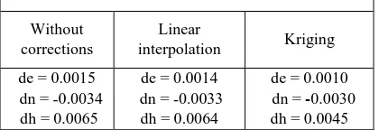
Table 4 demonstrates master-rover baseline values after relocating master station. In this table, three columns have been defined again. Note that after relocating and creating of zero difference observations, double differenced corrections generation algorithm which has been mentioned before, must be applied to the new relocated observations. In all of the cases new strategy has better performance in the height component. Zero difference VRS and the Kriging method has the best results.
Local value differences for RMRS - MICO baseline
Without corrections
Linear
interpolation Kriging de = 0.0015
dn = -0.0034 dh = 0.0065
de = 0.0014 dn = -0.0033
dh = 0.0064
de = 0.0010 dn = -0.0030
dh = 0.0045
Table 4. Master-Rover baseline processing accuracy after relocating master reference station
It is necessary to mention, in the both above strategies and their results, one can apply relative kinemtaic positioning in order to check coordinates of rover station in epochwisemode. Recommendation forfurtherreadingis Haji Mohammadloo, 2013.
CONCLUSION
In this paper a new NRTK method was presented. After formation of double differenced observations for each baselines in the network, ionospheric and tropospheric errors have been separated from each other. These corrections have been interpolated for the master-rover baseline. In order to reduce biases, two strategies have been introduced.In the first strategy the interpolated corrections are applied with negative sign to the single difference observations of master reference station. In the second numerical analysis, performance of the new virtual observation generation algorithm with applying Sagnac effect has been tested. In other words, the RINEX data of the master station is precisely re-located to the desired virtual station. Then double differenced interpolated corrections are applied to the virtual observations. The general performance of this strategy is better than the classical method. In this study kriging method has better results.
ACKNOWLEDGEMENTS
We would like to express our sincere thanks to Ms. Zangeneh-Nejad who devoted her time in the implementation of this project and development of the software.
REFERENCES
Asgari, J., 2005. “Etude de modèles Prédictifs Dans Un Réseau de Station GPS Permanent” Ecole Doctorale
Astronomie & Astrophysique D’Ile de France. Paris.
Asgari, J., Amiri-Simkooei, A.R., & Zangane-Nejad, F., 2011. A Virtual Reference Station Algorithm Development for a Network RTK System.
Blewitt, G., 1996. Basics of the GPS Technique: Observation
Equations. “Geodetic Applications of GPS” Basted, Sweden,
(Aug. 1996)
Chen, X., Han, S., Rizos, C., & Goh, P.C. 2000. Improving Real-time Positioning Efficiency Using the Singapore Integrated Multiple Reference Station Network (SIMRSN).
In: Proceedings of 13th International Technical Meeting of the Satellite Division of the U.S. Institute of Navigation, Salt Lake City, Utah, 19-22 September, 9-18.
Dai, L., Han, S., Wang, J., & Rizos, C., 2001. A Study on GPS/GLONASS Multiple Reference Station Techniques for Precise Real-time Carrier Phase-based Positioning. In: Proceedings of ION GPS 2001, 14th International Technical Meeting of Satellite Division of the Institute of Navigation, Salt Lake City, Utah, 11-14 September, pp. 392-403. Dai, L., Han, S., Wang, J., & Rizos, C., 2004. Comparison of Interpolation Algorithm in Network-Based GPS Techniques. In: Navigation, Journal of the Institute of Navigation. 50(4), pp. 277-293.
Fotopoulos, G., Cannon M.E., 2001. An Overview of Multi-Reference Station Methods for Cm-Level Positioning. GPS Solutions, 4(3), pp.1-10.
Haji mohammadloo, T., 2013. “Constrained Kinematic
Positioning” University of Isfahan. Isfahan.
Hofmann-Wellenhof, B., Lichtenegger, H., & Collins, J., 2007. Global Navigation Satellite System. GPS, GLONASS, GALILEO and More. Springer Wien, New York, pp. 161-272. Lachapelle, G., Alves, P., 2002. Multiple Reference Station Approach: Overview and Current Research. Journal of Global Positioning Systems. 1(2), pp. 133-136.
Leik, Al., 2004. GPS Satellite Surveying. John Wiley & Sons. New York.
Rizos, C., & Han, S., 2003. Reference Station Network Based RTK Sysems- Concepts and Progress. Wuhan University Journal of Natural Sciences, 8(2), 566-574.
Saeidi, A., 2012. “Evaluation of Network RTK in Southern Ontario” York University, Toronto.
Seeber, G., Satellite Geodesy: Foundations, Methods, and Applications. Hubert & Co. GmbH & Co. Kg. Gottingen. Berlin.
Wanninger, L., 1995. Improved Ambiguities Resolution by Regional Differential Ionosphere. In: Proceedings ION GPS-95, September 12-15, 19GPS-95, Palm Springs, pp. 55-62. Wanninger, L., 1999. The Performance of Virtual Reference Stations in Active Geodetic GPS-networks Under Solar Maximum Conditions. In: Proceedings of ION GPS-99, 12th
International Technical Meeting of the Satellite Division of the Institute of Navigation, Nashville, Tennessee, September 14-17: 1419-1427.
Wei, E., Chai, H., An, Z., & Liu, J., 2006. VRS Virtual Observations Generation Algorithm. Journal of Global Positioning Systems. 5(1-2), pp. 76-81.