A BREAKTHROUGH ENHANCEMENT OF FINITE ELEMENT METHOD
USING KRIGING INTERPOLATION
F.T. Wong
Assistant Professor at Department of Civil Engineering
Petra Christian University, Surabaya, Indonesia
ABSTRACT
During the last two decades, a large variety of mesh-free methods have been introduced as alternatives to the conventional finite element method (FEM). However, the acceptance in professional practices seems to be slow due to their implementation complexities. Recently, a convenient implementation of the element-free Galerkin method using Kriging interpolation (KI), which can be viewed as an enhancement of the FEM, was proposed. This method is subsequently referred to as Kriging-based FEM (K-FEM). In this method, field variables are approximated by “element-by-element” piecewise KI. Layers of finite elements around each element are adopted as its domain of influence (DOI). The distinctive advantage of the proposed method is its inheritance of the computational procedure of the FEM. Any existing FE code can be easily extended to K-FEM; thus, it has a higher chance to be accepted in the practice. This paper presents overview of the K-FEM. The formulation of KI and the concept of layered-element DOI are reviewed. The two-dimensional elastostatics problem is unitized as a vehicle to convey the concepts. Several examples are presented to demonstrate the reliability of the K-FEM.
Key words: finite element, Kriging interpolation, element-free Galerkin method
1. Introduction
The finite element method (FEM) is at present very widely used as a numerical method to solve various kinds of problems in engineering and science. The power and versatility of FEM have been tested for several decades of real engineering practices. One important issue in the FEM is mesh generation. Users often prefer to use the simplest elements, namely three-node triangular elements for two dimensional problems and four-node tetrahedral elements for three-dimensional problems, as they can be easily or even automatically generated and are more amenable to adaptive procedure. Nevertheless, it is well-known that these elements often give solutions of poor accuracy, in particular for the gradients of field variables such as stresses or stress resultants in solid and structural mechanics.
purpose FEM codes. Due to these inconveniences, these methods do not seem to find wide acceptance in real engineering practices.
In order to eliminate the aforementioned disadvantages, Plengkhom and Kanok-Nukulchai [6] proposed some modifications to the EFGM with moving Kriging interpolation (KI) [7]. The problem domain is subdivided into elements like in the conventional FEM. The KI is constructed for each element using a set of nodes in a domain of influence (DOI) composed of several layers of elements (the DOI is in the form of polygon for 2D problems). Combining the KI of all elements, the global field variable is thus approximated by piecewise KI. For evaluating the integration in the Galerkin weak form, the elements are employed as integration cells. This modified method can be viewed as an enhancement of the FEM using Kriging shape functions. Thus, this method was subsequently referred to as Kriging-based FEM (K-FEM) [8].
The K-FEM retains the advantages of mesh-free methods as follows [6]: 1) any requirement for high order shape functions can be easily fulfilled without any change to the element structure, 2) the field variables and their derivatives can be obtained with remarkable accuracy and global smoothness. A distinctive advantage of the K-FEM over other mesh-free methods is that it inherits the computational procedure of FEM so that existing general-purpose FE programs can be easily extended to include this new concept. Thus, the K-FEM has a higher change to be accepted in practices. The current research and development is the extension and application of the K-FEM to different problems in engineering, such as Timoshenko beam [9], general plate and shell structures [8, 10] and multi-scale mechanics [11].
This paper presents overview of the K-FEM. The formulation of KI and the concept of layered-element DOI are reviewed. The two-dimensional elastostatics problem is unitized as a vehicle to convey the concepts. Several examples are presented to demonstrate the reliability of the K-FEM.
2. Kriging Interpolation in the K-FEM
Named after Danie G. Krige, a South African mining engineer, Kriging is a well-known geostatistical technique for spatial data interpolation in geology and mining (e.g., see [12], [13]). Using this interpolation, every unknown value at a point can be interpolated from known values at scattered points in its specified neighborhood.
Formulation
Consider a continuous field variable u(x) defined in a domain Ω. The domain is represented by a set of properly scattered nodes xi, i=1, 2, …, N, where N is the total number of nodes in the whole domain. Given N field
values, u(x1), …, u(xN), the problem of interest is to obtain an estimate value of u at a point
x
0∈Ω
.The Kriging estimated value uh(x0) is a linear combination of u(x1), …, u(xn), i.e.
h
0 1
(
)
ni i( )
iu
x
=
∑
=λ
u
x
(1)where λi’s are termed as (Kriging) weights and n is the number of nodes surrounding point x0 inside a
sub-domain . This sub-domain is referred to as DOI in this paper. Considering individual function values, u(x
0
Ω ⊆ Ω
xh
0 1
(
)
ni i( )
iU
x
=
∑
=λ
U
x
(2)The Kriging weights are determined by requiring that the estimator Uh(x0) is unbiased, i.e. h
0 0
E
⎡
⎣
U
(
x
)
−
U
(
x
)
⎤
⎦
=
0
0
(3)
and by minimizing the variance of estimation error,
var
⎣
⎡
U
h(
x
0)
−
U
(
x
)
⎤
⎦
. Using the method of Lagrange for constraint optimization problems, the requirements of minimum variance and unbiased estimator lead to the following Kriging equation system:0
(
)
+
=
R
λ
P
μ
r x
(4a)T
0
(
)
=
P
λ
p x
(4b)in which 11 1 1
(
)
...
(
)
...
...
...
(
) ...
(
)
n n nC
C
C
C
⎡
⎤
⎢
⎥
= ⎢
⎥
⎢
⎥
⎣
⎦
h
h
R
h
h
n n; ; (4c)
1 1 1
1
( )
...
( )
...
...
...
(
) ...
(
)
m n mp
p
p
p
⎡
⎤
⎢
⎥
= ⎢
⎥
⎢
⎥
⎣
⎦
x
x
P
x
x
[
]
T1
...
nλ
λ
=
λ
;μ
=
[
μ
1...
μ
m]
T (4d)[
]
T0 10 20 0
(
)
=
C
(
)
C
(
) ...
C
(
n)
r x
h
h
h
;p x
(
0)
=
[
p
1(
x
0) ...
p
m(
x
0)
]
T (4e)R is
n
×
n
matrix of covariance between U(x) at nodes x1, …, xn; P isn m
×
matrix of polynomial values atthe nodes; λ is
n
×
1
vector of Kriging weights; μ ism
×
1
vector of Lagrange multipliers; r(x0) isn
×
1
vector of covariance between the nodes and the node of interest, x0; and p(x0) is vector of polynomial
basis at x
1
m
×
0. In Eqs. (4c) and (4e),
C
(
h
ij)
=
cov
⎡
⎣
U
( ), (
x
iU
x
j)
⎤
⎦
. Kriging weights λ can be obtained bysolving the Kriging equations, Eqs. (4a) and (4b).
The expression for the estimated value uh given by Eq. (1) can be rewritten in matrix form,
h T
0
(
)
u
x
=
λ
d
(5)where
d
=
[
u
( ) ...
x
1u
(
x
n)
]
T isn
×
1
vector of nodal values. Since the point x0 is an arbitrary point in theDOI, the symbol x0 can be replaced by symbol x. Thus, using the usual finite element terminology, Eq. (5) can
be expressed as
h
1
( )
( )
n i( )
ii
u
x
=
N x d
=
∑
=N
x u
(6)in which N(x)=λT(x).
Figure 1. Domain of influence for element el with one, two and three layers of elements [6]
Layered-Element Domain of Influence
Let us consider a 2D domain meshed with triangular elements, such as illustrated in Fig. 1. For each element, KI is constructed based upon a set of nodes in a polygonal DOI encompassing a predetermined number of layers of elements. The KI function over the element is given by Eq. (6). By combining the KI of all elements in the domain, the global field variable is approximated by piecewise KI. This way of approximation is very similar with the approximation in the conventional FEM.
It is worthy to note that it is also possible to use quadrilateral elements to implement the concept of layered-element DOI. Mesh with triangular layered-elements is a good choice owing to its flexibility in representing complex geometry and its ease to be automatically generated.
Within each element the interpolation function is naturally continuous. However, along the element edges between two adjacent elements the function is not continuous because the KI for the edge of each neighboring element is constructed using different set of nodes. Therefore, the present method is nonconforming. The issue of non-conformity and its effects on the convergence of the solutions obtained from the K-FEM were addressed in [14].
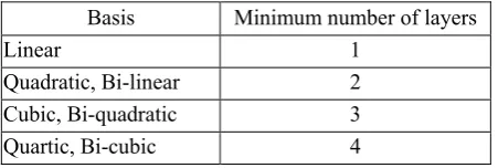
The number of layers for each element must cover a minimum number of nodes in such a way that the system of Kriging equations, Eqs. (4a) and (4b), can be solved. If an m-order polynomial basis is employed, the DOI is required to cover a number of nodes, n, that is equal or greater than the number of terms in the basis function [6]. Basically, it can be shown that the minimum number of layers for different polynomial bases is listed in Table 1. As the number of layers increases, the computational cost is higher. Thus the use of minimum number of layers for each polynomial basis is recommended.
Polynomial Basis and Correlation Function
Table 1. Minimum number of layers for various basis functions Basis Minimum number of layers
Linear 1
Quadratic, Bi-linear 2
Cubic, Bi-quadratic 3
Quartic, Bi-cubic 4
Covariance between a pair of random variables U(x) and U(x+h) can be expressed in terms of correlation coefficient function or shortly, correlation function, i.e.
ρ
( )
h
=
C
( ) /
h
σ
2, whereσ
2=
var
[
U
( )
x
]
. According to Gu [7], σ2has no effect on the final results and can be taken equals to 1. One of the widely used correlation model in the area of computational mechanics is the Gaussian correlation function ([6]-[11], [14]), viz.
2
( ) ( )h exp( ( h/ ) )
ρ
h =ρ
= −θ
d (7)where θ>0 is the correlation parameter,
h
=
h
, i.e. the Euclidean distance between points x and x+h, and d is a scale factor to normalize the distance. In this study, d is taken to be the largest distance between any pair of nodes in the DOI. Besides the Gaussian, we recently introduced the quartic spline (QS) correlation function ([8]-[10], [14]) as follows:2 3 4
1 6( / ) 8( / ) 3( / ) for 0 / 1 ( ) ( )
0 for / 1
h d h d h d h d
h
h d
θ
θ
θ
θ
ρ
ρ
θ
⎧ − + − ≤
= = ⎨
> ⎩
h ≤ (8)
Our studies showed that with this correlation function, Kriging shape functions are not very sensitive to the change in parameter θ. Moreover, the convergence characteristics of the K-FEM with the QS correlation function in many cases were more satisfactory than the Gaussian function.
Figure 2 shows the plot of the Gaussian and QS correlation functions for various values of θ. It can be seen that the parameter θ determines how quickly the correlation falls off; the larger value of θ, the quicker the correlation drops. For the same value of θ, the QS function drops quicker than the Gaussian function.
(a) (b)
Correlation Parameter
A proper choice of parameter θ is important as it affects the quality of KI. In order to obtain reasonable results in the K-FEM, Plengkhom and Kanok-Nukulchai [6] suggested a rule of thumb for choosing θ, i.e. θ should be selected so that it satisfies the lower bound,
10 1
1
1 10
n a i i
N
− + =− ≤ ×
∑
(9)where a is the order of basis function, and also satisfies the upper bound,
det( ) 1 10
R
≤ ×
−b (10)where b is the dimension of problem. For 2D problem with cubic basis function, for example, a=3 and b=2.
Numerical investigations on the upper and lower bound values of θ ([8], [10]) revealed that the parameter bounds vary with respect to the number of nodes in the DOI. Based on the results of the search for the lower and upper bound values of θ satisfying Eqs. (9) and (10), the author proposed explicit parameter functions for practical implementation of the K-FEM as follows:
For the Gaussian correlation parameter, the parameter function is
low up
(1 f) f
θ
= −θ
+θ
.8< ≤
< ≤ ≤
<
, 0≤ ≤f 0 (11a)
where f is a scale factor, θlow and θup are the lower and upper bound functions as follows:
low 2
0.08286 0.2386 for 3 10 -8.364E - 4 0.1204 0.5283 for 10 55
0.02840 2.002 for 55
n n
n n n
n n
θ
− ≤ ⎧ ⎪ =⎨ + − ≤⎪ + >
⎩
(11b)
up 2
0.34 0.7 for 3 10 -2.484E-3 +0.3275 0.2771 for 10 55
0.05426 7.237 for 55
n n
n n n
n n
θ
− ≤ ⎧ ⎪ =⎨ −⎪ + >
⎩
(11c)
For the QS correlation parameter, the parameter function can be obtained as
0.1329 0.3290 for 3 10 1 for 10
n n
n
θ
= ⎨⎧ − ≤≥
⎩ (12)
With these functions, adaptive values of θ can be used now in place of a uniform value of θ. Here, “adaptive” means that the correlation parameters used in an analysis are adjusted to the number of nodes in the DOI of each element. An advantage of the use of adaptive θ from practical viewpoint is that a user of K-FEM program is not required to input a value of θ in an analysis since its formulas can be embedded in the program.
Illustration
comprising one up to four element layers, are shown in the figure. It can be seen that the DOI is not necessary to be convex.
Figure 3. Square domain with triangular elements and various layered-element domains of influence
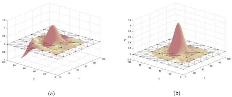
Now suppose we use quadratic basis function (m=6) and three element layers to construct KI over Element no.1. In this case the DOI encompasses the nodes in the 1st, 2nd and 3rd layers and the total number of the nodes is 30 (n=30) as may be illustrated in Fig. 3. Hence it satisfies the requirement . The plot of Kriging shape functions associated with node I, using Gaussian and QS correlation functions, is shown in Fig. 4. The correlation parameters were taken in such a way so that they are in the middle between their lower and upper bounds (Eqs. (9) and (10)), i.e. θ=4.2 for the Gaussian and θ=1.5 for the QS. One can observe that the shape function with QS correlation function is relatively more flat in the region far from the node under consideration (Node I).
n
≥
m
(a) (b)
Figure 4. Kriging shape functions corresponding to node I using: (a) Gaussian correlation function, (b) quartic spline correlation function
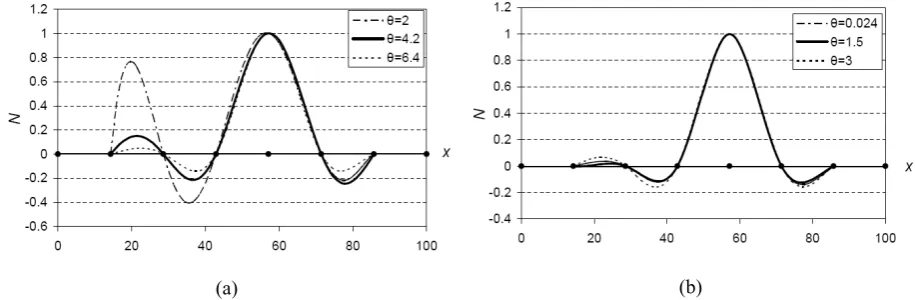
boundary of the DOI. On the other hand, the QS shape function is not very sensitive to the change of θ. The functions for different values of θ are nearly the same, except in regions close to the boundary of the DOI. From practical point of view, the insensitivity of the shape function to the parameter θ is an advantage since a user of the K-FEM does not have to consider which value of θ should be used in the analysis.
(a) (b)
Figure 5. Kriging shape functions corresponding to node I along line y=57.14, using: (a) Gaussian correlation function, (b) quartic spline correlation function
3. Formulation of the K-FEM for 2D Elastostatics
The governing equations for 2D elastostatics in Cartesian coordinate system can be written in a weak form as follows:
T T
V
δ
dV
=
Vδ
dV
+
Sδ
dS
∫
ε σ
∫
u b
∫
u t
T (13)where
u
=
{
u
v
}
T is the displacement vector;ε
=
{
ε
xε
yγ
xy}
T is the vector of 2D strain components;{
}
Tx y xy
σ
σ
τ
=
σ
is the vector of 2D stress components;b
=
{
b
xb
y}
T is the body force vector;{
}
Tx y
t
t
=
t
is the surface traction force vector; V is the 3D domain occupied by the solid body and S is thesurface on which the traction t is applied.
Suppose the domain V is subdivided by a mesh of Nel elements and N nodes. To obtain an approximate solution
using the concept of KI with layered-element DOI, for each element e=1, 2, …, Nel the displacement components u and v are approximated by the KI as follows:
1
( , ) n i( , ) i
i
u x y
∑
= N x y u ; (14)1
( , ) n i( , ) i
i
v x y
∑
= N x y vHere, Ni(x, y) denotes Kriging shape function associated with node i; ui and vi are nodal displacement
components in the x and y directions, respectively; n is the number of nodes in the DOI of an element, which generally varies from element to element. In the matrix form, Eq. (14) may be written as
e
=
eu
N r
e (15a)1 2
1 2
0
0
0
0
0
n e
n
N
N
N
N
N
⎡
⎤
= ⎢
⎥
⎣
⎦
N
"
"
0
N
(15b)is the shape function matrix and
{
}
T1 1 2 2
e
n n
u
v
u
v
u
v
=
r
"
(15c)is the element nodal displacement vector. The variable index e is written to emphasize that the matrices are associated with element e, , and follow the local (elemental) ordering of element e. Employing the small-strain strain-displacement relation and linear stress-strain relation and inserting the element-by-element approximation of u, Eq. (15a), into the weak form, Eq. (13), we obtain
el
1
≤ ≤
e
N
el T T el T T el T T
1
(
e)
1 e 1N e e e e N e e e N e e e
e=
δ
VdV
=
e=δ
VdV
+
e=δ
dS
∑
r
∫
B EB
r
∑
r
∫
N b
∑
r
eN t
S
∫
0
n yN
(16)In this equation, Be is the element strain-displacement matrix, i.e.
1, 2, ,
1, 2, ,
1, 1, 2, 2, , ,
0
0
0
0
0
x x n x
e
y y
y x y x n y n x
N
N
N
N
N
N
N
N
N
N
N
⎡
⎤
⎢
⎥
= ⎢
⎥
⎢
⎥
⎣
⎦
B
"
"
"
(17)Matrix E is the constitutive matrix, which for the case of isotropic material can be expressed in terms of modulus elasticity E and Poisson’s ratio ν as follows:
2
1
0
1
0
1
0
0
(1
) / 2
E
ν
ν
ν
ν
⎡
⎤
⎢
⎥
=
⎢
⎥
−
⎢
−
⎥
⎣
⎦
E
(18a) in which 2(1
)
E
E
E
ν
⎧
= ⎨
−
⎩
and(1
)
ν
ν
ν
ν
⎧
= ⎨
−
⎩
for plane stress
for plane strain
(18b)Ve is the 3D domain of element e and Se is the surface of element e on which the traction t is applied. Since Eq. (16) must be true for any admissible virtual displacement δre, we can write the equilibrium equation for each element as follows:
e e
=
ek r
R
(19a)where
T T
e e
e e e e e e
V
dV
t
AdA
=
∫
=
∫
k
B EB
B EB
(19b)is the stiffness matrix of element e (the matrix dimension is
2
n
×
2
n
);T T T
e e e e
e e e e e e e e e e e
V
dV
SdS
t
AdA t
sds
=
∫
+
∫
=
∫
+
∫
R
N b
N t
N b
N t
T1
(19c)
In view of global (structural) ordering, the summation in Eq. (16) is equivalent to the finite element assembly procedure. Hence, from Eq. (16) we can obtain the global discretized equilibrium equations
=
Kr
R
(20a)in which el 1 N e e=
= Α
K
k
; ; (20b)el 1 N e e=
= Α
r
r
el 1 N e e== Α
R
R
Here K is the structural stiffness matrix (
2
N
×
2
N
); r is the structural nodal displacement vector (2
N
×
1
);R is the structural nodal force vector (
2
N
×
1
), andel
1
N
e
Α
= denotes the assembly operator. It should be mentionedhere that the assembly process for each element involves all nodes in the element’s DOI, not only the nodes within the element as in the conventional FEM.
Solving Eq. (20a), one can obtain r and once it is known, one can extract element nodal displacement, re, for each element. Stresses in each element can then be calculated by the use of the following equation:
e
=
eσ
EB r
e (21)Matrix Be in this equation is a function of the coordinates and must be evaluated at the locations in the element where the stresses are desired. In the following examples, the stresses are evaluated at the element nodes for every element. Subsequently, at nodes where two or more elements meet the element nodal stresses are averaged.
It is worthwhile to note that the interpolation function for calculation of the stresses do not have to be the same as that used for constructing the stiffness matrix. For example, if the KI employed to construct the stiffness matrix is Kriging with the options of quadratic basis, two-element-layer DOI, QS correlation function (P2-2-QS), the KI in evaluating the stresses may be with the options of cubic basis, three element-layers, Gaussian correlation function (P3-3-G). It is also possible to use the constant-strain- triangle interpolation function for calculation of the stresses. In the following examples, however, the interpolation function for calculation of the stresses is taken to be the same as that used for constructing the stiffness matrix.
4. Numerical Tests
To study the accuracy and convergence of the present K-FEM, two measures of errors are utilized. The fist one is the relative error of displacement norm, defined as
1 2 app exact T app exact
exact T exact
(
) (
)
(
)
V u VdV
r
dV
⎛
−
−
⎞
⎜
⎟
=
⎜
⎟
⎝
⎠
∫
∫
u
u
u
u
u
u
(22)
where uapp and uexact are the approximate and the exact displacement vectors, respectively. The second one is the relative error of strain energy norm, defined as
1 2 app exact T app exact
exact T exact
(
)
(
)
(
)
V VdV
r
dV
ε⎛
−
−
⎞
⎜
⎟
=
⎜
⎟
⎝
⎠
∫
∫
ε
ε
E
ε
ε
where εapp and εexact are approximate and exact strain vectors, respectively. For computing these relative errors, the 13-point quadrature rule for triangles (see e.g. [15: p.173]), which can give error figures of four digits accuracy, is employed.
The element stiffness matrix, Eq. (19b), is computed using the 6-point quadrature rule for triangles. The 6-point rule is selected because it can give reasonably accurate results (three digits accuracy in most cases) yet inexpensive in terms of computational cost. For computing the nodal force vector, Eq. (19c), the 2-point Gaussian quadrature for line integral is used since it results in exact nodal force vector for edge traction force with cubic distribution or less.
Abbreviations in the form of P*-*-G* or P*-*-QS, in which the star denotes a number, are adopted in this section to designate various options of the K-FEM. The first part of the abbreviation denotes polynomial basis with the order indicated by the number next to letter P; the middle part denotes number of layers; the last part, G* denotes the Gaussian correlation function with the adaptive parameter given by Eq. (11a) and with the scale factor f indicated by the number next to letter G (in percent); QS denotes the quartic spline correlation function with the adaptive parameter given by Eq. (12). For example, P3-3-G50 means cubic basis, 3 element-layers, Gaussian correlation function with mid-value parameter function, i.e. f=0.5.
A Cantilever Plane Stress Beam Example
A cantilever plane stress beam of one unit thickness subjected to parabolic end shear traction as shown in Fig. 6. The analytical solutions for this problem are as follows [16]:
(
) [ 3 (2
) (2
) (
6
2
P
D
u
y
x
L
x
y y
EI
ν
= −
−
− + +
−
D
) ]
(24a)2 2
4 5
[
(3
) 3 (
)(
)
6
2
P
D
v
x
L
x
L
x y
D
EI
2
]
4
x
ν
ν
+
=
− +
−
−
+
(24b)(
)(
2
xP
D
L
x y
I
σ
= −
−
−
)
;σ
y=
0
;(
)
2
xyPy
y
D
I
τ
= −
−
(24c)where I=D3/12 .
Figure 6. A cantilever beam subjected to parabolic shear
To study the convergence of the K-FEM with various options, the beam is modelled with different degrees of mesh refinement. The initial course mesh with 24 nodes (the element characteristic size h=1) is shown in Fig. 7. Subsequent meshes are constructed by subdividing the previous element into four smaller elements. The refined meshes considered in this test are meshes with h=0.5 (77 nodes), h=0.25 (273 nodes), and h=0.125 (1025 nodes). The K-FEM options used for analyses of the beam and the other following problems are: P2-2-G80, P2-2-QS, P3-3-G80, and P3-3-QS.
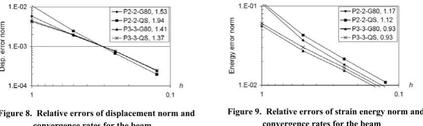
Plots of relative error norms for displacement and strain energy and their convergence rates are shown in Figs. 8 and 9, respectively. The fastest convergence rate for displacement is achieved for the K-FEM with P2-2-QS (the convergence rate R=1.94). The three other options result in nearly the same rate (around 1.5). In terms of strain energy error norm, all of the K-FEM options converge with nearly the same convergence rate (around 1). The K-FEM with P3-3-G80 is the most accurate one. It is worthwhile to note that in this problem the K-FEM with cubic polynomial basis should theoretically reproduce the exact solutions because the order of the exact solutions is three. However this is not the case here because of inter-element non-conformity of the K-FEM with P3-3.
Figure 8. Relative errors of displacement norm and convergence rates for the beam
Figure 9. Relative errors of strain energy norm and convergence rates for the beam
The contours of the normal stress in x direction, σx, and the shear stress, τx, without averaging process, are
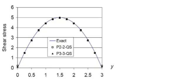
displayed in Fig. 10 for the mesh with h=0.5 and the K-FEM options P3-3-QS. These plots demonstrate the capability of the K-FEM to produce smooth stress distributions in a relatively course mesh. The average nodal shear stresses of the beam at the mid-span are shown in Fig. 11 for the mesh with h=0.25 and the options P2-2-QS and P3-3-P2-2-QS. The figure demonstrates the accuracy of the method in computing the shear stress, which is generally hard to obtain for the standard FEM. The K-FEM with P3-3-QS is slightly more accurate than that with P2-2-QS, particularly at the edges of the beam.
(a) Normal stress, σx (b) Shear stress, τxy
Fig. 11 Average shear stresses at the mid-span of the cantilever beam with mesh of h=0.25
An Infinite Plate with a Hole
An infinite plane-stress plate with a circular hole of radius a=1 is subjected to a uniform tension Tx=100 at
infinity [17] (Fig. 12). The exact stress fields in the plate are given as follows [16]:
2 4
2 4
3
3
1
cos 2
cos 4
cos 4
2
2
x x
a
a
T
r
r
σ
=
⎡
⎢
−
⎛
⎜
θ
+
θ
⎞
⎟
+
⎤
⎝
⎠
⎣
θ
⎦
⎥
(25a)2 4
2 4
1
3
cos 2
cos 4
cos 4
2
2
y x
a
a
T
r
r
σ
=
⎡
⎢
−
⎛
⎜
θ
−
θ
⎞
⎟
−
⎤
⎝
⎠
⎣
θ
⎦
⎥
(25b)2 4
2 4
1
3
sin 2
sin 4
sin 4
2
2
xy x
a
a
T
r
r
τ
=
⎡
⎢
−
⎛
⎜
θ
+
θ
⎞
⎟
+
⎤
⎝
⎠
⎣
θ
⎦
⎥
(25c)where r and θ are the polar coordinates and θ is measured from the positive x-axis counter-clockwise. Owing to symmetry, only the upper right quadrant of the plate,
0
≤ ≤
x
5
and0
≤ ≤
y
5
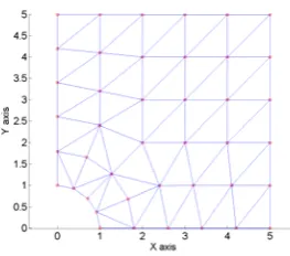
, is analyzed. Zero normal displacements are prescribed on the symmetric boundaries and the traction boundary conditions given by the exact stress, Eqs. (25a)-(25c), are imposed on the right (x=5) and top (y=5) edges.The initial course mesh of 42 nodes is shown in Fig. 13. The element characteristic size for this problem is taken as the distance between two nodes at the right or top edge, i.e. h=1. Subsequently, the mesh is refined by subdividing the previous element into four smaller elements. The refined meshes considered in this test are meshes with h=0.5 (141 nodes) and h=0.25 (513 nodes). In performing the analysis with h=0.25 using Gaussian correlation function, the scale factor f=0.79 is used in place of f=0.8 because the use of f=0.8 results in det(R) exceeding the upper bound criterion, Eq. (10), for some elements.
The contour of the un-averaged normal stress in x direction, σx, for the plate with mesh of h=0.5 and the option
P3-3-QS is shown in Fig. 16. Again, it demonstrates the capability of the present method to produce smooth stress distribution even for a rather crude mesh.
Figure 12. An infinite plate with a circular hole
Figure 13. Initial mesh of the holed plate
Figure 14. Relative errors of displacement norm and convergence rates for the holed plate
Figure 15. Relative errors of strain energy norm and convergence rates for the holed plate
Figure 16. Contour of un-averaged σx for the holed plate discretized with 141 nodes, computed using the K-FEM with
option P3-3-QS
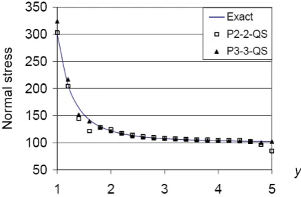
The average nodal stresses σx along x=0 are depicted in Fig. 17 for the mesh with h=0.25 for two options:
but there are some fluctuations at the region near the peak stress and at the boundary y=5. The K-FEM with P3-3-QS captures better the steep stress distribution near the peak stress.
Figure 17. Normal stress in the x-direction along line x=0 of the holed plate with mesh of h=0.25
5. Conclusions
The fundamentals of the K-FEM and its application to two-dimensional elastostatics have been presented. The basic concepts are applicable to many problems in continuum mechanics. Besides the commonly-used Gaussian correlation function, the QS function is introduced as an alternative for the correlation model. The advantage of the use of the QS is that the shape functions are not very sensitive to the change of the parameter. The numerical tests with two benchmark problems in plane-stress/plane-strain problems demonstrate the superior convergence and accuracy of the method.
The present method is as simple as the conventional FEM in terms of the formulation and implementation yet it is as flexible as mesh-free methods. The drawback of the present method is that it is non-conforming along inter-element boundaries. However, despite the non-conformity, the numerical examples showed very good convergence characteristics. Future researches may be directed at: (1) extension and application of the K-FEM to different problems in engineering, (2) inclusion of adaptive mesh refinement, (3) improvement of the computational efficiency in constructing Kriging shape functions.
6. References
1) Belytschko, T., Krongauz, Y., Organ, D., Fleming, M., and Krysl, P. (1996). ‘Meshless Methods: An Overview and Recent Developments’, Computer Methods in Applied Mechanics and Engineering, 139, 3-47.
2) Liu, G.R. (2003). Mesh Free Methods. Boca Raton: CRC Press.
3) Fries, T. P. and Matthies, H. G. (2004). Classification and Overview of Meshfree Methods. Brunswick, Germany: Institute of Scientific Computing, Technical University Braunschweig.
4) Gu, Y.T. (2005). ‘Meshfree Methods and Their Comparisons’, International Journal of Computational Methods, 2, 477-515.
6) Plengkhom, K. and Kanok-Nukulchai, W. (2005). ‘An Enhancement of Finite Element Methods with Moving Kriging Shape Functions’, International Journal of Computational Methods, 2, 451-475.
7) Gu, L. (2003). ‘Moving Kriging Interpolation and Element-Free Galerkin Method’, International Journal for Numerical Methods in Engineering, 56, 1-11.
8) Wong, F.T. and Kanok-Nukulchai, W. (2006). ‘Kriging-based Finite Element Method for Analyses of Reissner-Mindlin Plates’, in W. Kanok-Nukulchai, S. Munasinghe and N. Anwar Eds., Emerging Trends: Keynote Lectures and Symposia, Proceedings of the Tenth East-Asia Pacific Conference on Structural Engineering and Construction (EASEC-10), 3-5 August 2006, Bangkok, Thailand, Asian Institute of Technology, pp. 509-514.
9) Wong, F.T. and Syamsoeyadi, H. (2011). ‘Kriging-based Timoshenko Beam for Static and Free Vibration Analyses’, Civil Engineering Dimension, 13, 42-49. Surabaya, Indonesia: Petra Christian University. 10) Wong, F.T. (2009). ‘Kriging-based Finite Element Method for Analyses of Plates and Shells’, Asian
Institute of Technology Dissertation No. St 09 01. Pathumthani, Thailand: Asian Institute of Technology. 11) Sommanawat, W. and Kanok-Nukulchai, W. (2009). ‘Multiscale Simulation Based on Kriging-Based
Finite Element Method’, Interaction and Multiscale Mechanics, 2, 387-408.
12) Olea, R.A. (1999). Geostatistics for Engineers and Earth Scientists. Boston: Kluwer Academic Publishers. 13) Wackernagel, H. (1998). Multivariate Geostatistics, the 2nd, completely revised edition. Berlin: Springer. 14) Wong, F.T. and W. Kanok-Nukulchai (2009). ‘On the Convergence of the Kriging-based Finite Element
Method’, International Journal of Computational Methods, 6, 1-27.
15) Hughes, T. J. R. (1987). The Finite Element Method: LinearStatic and Dynamic Finite Element Analysis. New Jersey, USA: Prentice-Hall.
16) Atluri, S. N., Zhu, T. (2000). ‘New concepts in meshless methods’, International Journal for Numerical Methods in Engineering, 47, 537-556.
![Figure 1. Domain of influence for element el with one, two and three layers of elements [6]](https://thumb-ap.123doks.com/thumbv2/123dok/1579684.2053595/4.595.161.443.102.256/figure-domain-influence-element-el-layers-elements.webp)