Directory UMM :Data Elmu:jurnal:M:Mathematical Social Sciences:Vol39.Issue1.Jan2000:

www.elsevier.nl / locate / econbase

Price volatility and risk with non-separability of preferences

a b ,_*

Burkhard Drees , Bernhard Eckwert a

International Monetary Fund, Research Department, Washington, DC 20431, USA b

Department of Economics, University of Chemnitz, D-09107 Chemnitz, Germany

Received 1 April 1998; received in revised form 1 August 1998; accepted 1 September 1998

Abstract

This paper studies the relationship between the systematic risk of financial instruments and the volatility of their equilibrium prices in a two-period stochastic asset valuation model. Whereas there is no link between the relative risk of assets and their price volatility in standard representative-agent models with additively-separable preferences, in this model with non-separable preferences a riskier asset can have higher or lower price volatility than a safe asset depending on the intertemporal changes in risk aversion. If individual preferences exhibit risk substitutability (i.e. future relative risk aversion decreases with higher current consumption), then the riskier asset has a more volatile price than the less risky asset. Agents’ risk complementarity (i.e. increasing future relative risk aversion with higher current consumption), on the other hand, implies an inverse relationship between the relative riskiness of assets and the volatility of their prices.  2000 Elsevier Science B.V. All rights reserved.

Keywords: Price volatility; Risk; Assets

JEL classification: E31

1. Introduction

The contribution of this article is to show how the random behavior of equilibrium asset prices depends on the assets’ riskiness. The relation between risk and asset prices has long been the subject of both theoretical and empirical research in financial economics. While a major part of the recent literature is concerned with the impact of the stochastic nature of the dividend process on stock price variability, our analysis addresses the question how the systematic risk of an asset, as measured by its

*Corresponding author. Tel.:149-0371 / 531-4230; fax:149-5313970. E-mail address: b.eckwert@wirtschaft.tu-chemnitz.de (B. Eckwert)

equilibrium conditional risk premium, translates into price volatility. How is the relative price volatility of two assets related to their relative riskiness? Or, more concretely, does the market price of a risky asset exhibit larger volatility than the price of a relatively safe asset?

It appears that conventional asset pricing theory suggests a positive relationship between risk and price volatility. The argument could run as follows: the riskiness of an asset, as measured by its equilibrium risk premium, is closely related to the degree of individual risk aversion. In general, higher risk aversion leads to a higher risk premium. Furthermore, as has been shown by LeRoy and LaCivita (1981) et al., consumption-based asset pricing models imply a positive relationship between individual risk aversion and the volatility of equilibrium asset prices. Thus, the size of the price fluctuations on the stock market appears to be positively related to the riskiness of the assets.

However, since this argument is comparative static in nature, it is not applicable to economies in which many financial assets with different risk characteristics are traded at the same time. In other words, this argument is not helpful in explaining the impact of the risk structure across assets on the joint stochastic behavior of their equilibrium prices. To the extent that this impact is significant, the aggregation of the stock market in the conventional intertemporal asset pricing approach is not an innocuous simplification; rather it may account for both the excess volatility of prices found in recent empirical studies (e.g. Pontiff, 1997, Shiller, 1989) as well as the empirical fact that the ‘price of risk’ is not common across countries (Bekaert and Harvey, 1997; King et al., 1994).

This paper is complementary to the work by Abel (1988), Giovannini (1989), and Poterba and Summers (1986) who investigate stock price responses to changes in dividend payments. One of the main lessons to be learned from the CAPM model is that, in general, an increase in dividend volatility is not equivalent to an increase in the riskiness of an asset as measured by the risk premium. The market does not reward total risk but systematic risk, which is the non-diversifiable risk component of an asset’s return. While the total risk of an asset depends on the volatility of its payoffs, the non-diversifiable risk depends also on the covariances between this asset’s return and the payoffs of all other assets which are traded. Highly volatile returns that are uncorrelated or even negatively correlated with the market will not be perceived as risky by well diversified investors. Thus, the analysis by Abel, Giovannini, and Poterba and Summers sheds no light on the issue of how the systematic risk of a financial instrument translates into price volatility.

Our theoretical setup is a simple two-period exchange economy with one perishable consumption good and two assets that can be used to transfer wealth into the future. The payoffs of both assets are stochastic. The analysis shows that the agents’ attitudes towards risk are critical in determining the relation between the relative riskiness of a financial instrument and the relative dispersion of its price. If individual preferences exhibit risk substitutability, i.e. if the degree of future period relative risk aversion is a decreasing function of first period consumption, then higher relative risk of an asset corresponds to greater asset price volatility. In case of risk complementarity, i.e. when future period relative risk aversion depends positively on current consumption, the variability of the equilibrium asset prices is inversely related to the risk of the financial instruments.

The key assumption is non-time-separability of preferences. If preferences are additively time-separable, the volatility of asset prices does not depend on their relative risk. Thus a Lucas (1978)-type representative consumer asset pricing model with additively time-separable preferences is not flexible enough to capture the impact of the intertemporal substitution effects of marginal utility on the relation between asset price variability and risk. Mehra and Prescott (1973) provide strong evidence against the standard representative consumer model of asset pricing and blame the rigid additively time-separable specification of preferences for the dramatic failure to generate an equity premium of an empirically plausible magnitude.

The paper proceeds as follows: Section 2 describes the economic environment and defines equilibrium prices; in Section 3 we define a concept of asset price dispersion and relate it to the assets’ risk characteristics. Concluding remarks are presented in Section 4, and some proofs are gathered in Appendix A.

2. The model

Consider a two-period economy with one perishable consumption good (numeraire) and two financial assets, p and q. The assets’ payoffs, h( y ) and g( y ), depend on at t

]

stochastic signal yt[[y, y],IR which becomes public information at the beginning of

1 ]

period t51, 2. Assuming that the distribution of y does not depend on the realization2

of y , the cumulative distribution function of y is F. We restrict F to be an element of1 2

]

the setF of all strictly increasing cumulative distribution functions on [y, y]. h and g are

]

strictly positive differentiable functions with h±ag ;a .0 (no redundancy). Without

]

loss of generality, we assume that (≠/≠y)[h( y)1g( y)]$0 ;y[[y, y]. The time 1

p q]

ex-dividend prices of the assets p and q are denoted by p and p .

The economy is populated by a representative individual who owns one share of each asset at the beginning of period 1. After observing the state y , the agent receives all1

dividends and uses them to buy consumption goods and additional shares to be carried over into the next period. In the final period, he spends all dividends from his share holdings on consumption. Thus the agent’s choices are constrained by

1

p q

c1p (z21)1p (s21)5h( y)1g( y) (1)

˜ ˜ ˜

c5zh(y )1sg(y ) (2)

c denotes the agent’s consumption in the first period; z and s are the holdings of assetsp

and q at the end of the first period. A tilde marks variables which refer to the second period and are unknown in period 1.

We assume that the agent’s preferences over random lifetime allocations can be described by the expected value of a thrice differentiable intertemporal utility function

˜

EhU(c, c )j; Ui.0, Uii,0 for i51,2, U21.0, lim U15lim U25 ` (3)

c→0 ˜c→0

where E is the expectations operator conditional on the first period information set. This specification of individual preferences is standard. The assumption that U21 is greater than zero means that the consumer views present and future consumption as

comple-2

ments so that the marginal utility of c is higher for larger c , and vice versa.2 1

In order to keep the analysis as general as possible we will use risk and volatility concepts that are largely independent of the parameters of the model (preferences, probabilistic specification). In particular, these concepts (and hence the characterization of the risk-volatility link) will not be affected by the choice of F[F and by the specification of the investor’s preferences as long as Eq. (3) is satisfied.

The equilibrium ex-dividend prices in period 1 depend on the state variable y,

p p q q

p 5p ( y), p 5p ( y). If the agent knows the distribution of dividend payments, then

the necessary and sufficient conditions for his decision problem are

p _{˜ ˜ ˜}

p ( y)EhU (c, c )1 j5EhU (c, c )h(y )2 j (4)

q

˜ ˜ ˜

p ( y)EhU (c, c )1 j5EhU (c, c )g(y )2 j (5) These equations state that, at an optimum, investing one unit of consumption in any asset and consuming the proceeds in period 2 should not, on average, increase utility compared to consuming that unit at time 1. Using the market clearing conditions

z5s51, the consumer’s first-order conditions are

p

˜ ˜ ˜ ˜ ˜ ˜ ˜

p ( y)

E

U (c( y), c(y )) dF(y )1 5

E

U (c( y), c(y ))h(y ) dF(y )2 (6)

q

˜ ˜ ˜ ˜ ˜ ˜ ˜

p ( y)

E

U (c( y), c(y )) dF(y )1 5

E

U (c( y), c(y ))g(y ) dF(y )2 (7) where

˜ ˜ ˜ ˜ c( y)[h( y)1g( y), c(y )[h(y )1g(y ). 2

p

Definition 2.1. An equilibrium is a pair of strictly positive price functions p (?) and

q

p (?) such that Eq. (6) and Eq. (7) are satisfied for all y.

Because of the simple structure of our economy, the equilibrium price functions are directly determined by Eqs. (6) and (7).

3. The risk structure of financial assets and the volatility of equilibrium prices

The systematic risk of an asset is measured by its equilibrium risk premium, which depends on the realized state in period one, on the distribution F[F of the signal y ,2

and on the specification of the investor’s preferences. That is, the riskiness of asset p

does not need to be comparable to the riskiness of asset q if, for example, the former pays a higher risk premium in some states of nature at time 1 and a lower risk premium in others. Our strategy is to characterize the relative price volatility of assets with payoff patterns that can be ranked according to their systematic risks. More precisely, we concentrate on the subclass of all asset return functions for which a robust (with respect to the state at time 1 and the parameterization of the economy) risk ordering exists and relate the riskiness of the assets to the relative volatility of their equilibrium prices. Consider the expected real rates of return,

˜ ˜

Ehh(y )j Ehg(y )j

]]] ]]]

r ( y)p [ p , r ( y)q [ q

p ( y) p ( y)

The difference between the real rates of return, r( y)[r ( y)p 2r ( y), equals theq

difference between the conditional risk premia of both assets and is a convenient measure of relative risk.

Definition 3.1. Asset q is said to be riskier (less risky) than assetp, q.rp(p .rq), if,

]

for any y[[y, y], any F[F, and any utility function U which satisfies Eq. (3), asset q

] (.)

pays a higher (lower) conditional risk premium than asset p: r( y) 0;y, given any

,

admissible F and U.

For the subsequent analysis it is convenient to normalize the asset returns by defining

3

ˆ ˜ ˜ ˜ ˆ ˜ ˜ ˜

h(y )[h(y ) /Ehh(y )j and g(y )[g(y ) /Ehg(y )j. Proposition 3.1 provides a complete

ˆ _ˆ

characterization of the properties of the normalized return functions h and g that allow a comparison of the risk of assetsp and q in the sense of Definition 3.1.

ˆ ˜ ˆ ˜ ˜

Proposition 3.1. Let s(y )[g(y )2h(y ) be the difference between the normalized

returns on assets q and p. Asset q is riskier (less risky) than asset p, if and only if

3

˜y

]

($)

˜ ˜

S(y; F )[

E

s( y9) dF( y9)_#0 ;y[[y, y], ;F[F

]

y

]

Proof. See Appendix A.

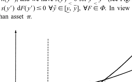
The class of comparable assets characterized in the above proposition includes those

˜ ˜ ˜

pairs of assets q and p for which r(y )[g(y ) /h(y ) is strictly monotone. If, for

]

˜ *

example, r(y ) is strictly increasing, then there exists a unique y [[y, y] with

]

(.) (.)

ˆ ˜ ˜ ˜ ˜

ˆ * * *

g( y )5h( y ), and we have s(y ) 0 for y y (see Fig. 1) and Ehs(y )j50. Thus S(y;

, ,

˜y _]

˜

F )5ey s( y9) dF( y9)#0 ;y[[y, y], ;F[F. In view of Proposition 3.1, asset q is

]

]

[image:6.612.110.363.249.406.2]

riskier than asset p.

Fig. 1. Normalized asset payoffs.

To relate the systematic risk of assets to the fluctuations of their equilibrium prices, an operational concept of price volatility is needed. This concept, which will be stated in

p q

detail below, says roughly the following: If two asset prices, p and p , have the same mean and if for some state y and any realization y in a neighbourhood of y the price0 0

p p q q p

p ( y) is more distant from p ( y ) than p ( y) is distant from p ( y ), then p0 0 is more

q p

volatile than p at y . In other words, the asset price p0 is said to be more volatile than

q p q p

the asset price p at y , expressed as p0 .y_op , if, after normalization, p spreads

q

locally more widely around its value at y than p .0

For any positive random variable v defined on the real line, let v(?; x,h) be the

normalized (unit mean) restriction of v to the interval A(x,h)_[[x2h, x1h],

v(?; x,h)_[v(?)u

Y E

v( y) dF( y) A(x,h)

A(x,h)

p q p q

p p q q

up ( y; y ,h)2p ( y ; y ,h)u.up ( y; y ,h)2p ( y ; y ,h)u, y ±_y

0 0 0 0 0 0 0

[A( y ,0 h) (8)

p q p q

p is said to be more volatile than p , p .volp , if Eq. (8) holds for all y .0

Whereas Proposition 3.1 relates the relative riskiness of an asset to the fundamentals of the model, the next proposition describes the link between fundamentals and asset price volatility.

4

˜

Let R denote the relative risk aversion in the future period,

˜ ˜ U (c, c )c22

˜ _{˜ ]]]}

R(c, c )[2 _˜

U (c, c )2

Proposition 3.2. The ordering of the financial assets with respect to the volatility of

˜ their equilibrium prices depends on the relative risk aversion in the second period, R(?,

˜

?), and on the difference s(y ) between the normalized asset returns:

5 _˜

˜

(i ) Suppose R(c, c ) is strictly decreasing in c. Then

q p

p s_{p if S#0} vol

.

p q

5

p s_{p if S$0} vol

˜ _˜

(ii ) Suppose R(c, c ) is strictly increasing in c. Then

p q

p s_{p if S#0} vol

.

q p

5

p s_{p if S$0} vol

Proof. See Appendix A.

The relative price volatilities of the two assets depend on the properties of the return functions g and h, as summarized by the sign of S, and on the impact of higher current consumption on the individual’s attitudes towards future risk. If individual preferences

˜ _˜

are such that R(c, c ) is strictly monotone in c, then Propositions 3.1 and 3.2 indicate that within the class of risk-comparable assets both the relative risk and the relative price

4

The classical theory of portfolio selection based on the work by Arrow (1970) and Pratt (1964) is concerned with the optimal composition of a portfolio of a given size. This approach deals with choices between timeless uncertain prospects, i.e. the individual investor simply maximizes the expected utility of his final wealth w, and his attitudes towards risk can be characterized in terms of a risk aversion function depending on w. In our integrated model of saving and portfolio choice the size and the composition of the portfolio are simultaneously determined, so that the uncertain prospects become temporal. The appropriate risk aversion function for such prospects measures the willingness to bear temporal risks and is derived from the measure suggested by Arrow and Pratt by replacing the marginal utility of wealth with the marginal utility of future consumption (for a proof and a more extensive discussion of portfolio decisions under timeless and temporal

`

risks see Dreze and Modigliani, 1972).

5 ]

We use the notational convention S#0⇔S( y)#0;y[[y, y],;F[F. In addition, by ‘strictly increasing ]

volatility of the assets can be parameterized by the sign of S. Thus, within the class of all assets which can be ranked with respect to their risks, we can use this parameterization to relate the price volatility of an asset to the riskiness of its payoff pattern. First consider the case where risk aversion in the second period is a strictly decreasing function of first period consumption. Propositions 3.1 and 3.2 imply

q p

˜ _˜

R(c, c ) is strictly p s_{p and q. p if S#0} r

vol

⇒

5

p q (9)

decreasing in c p s_{p andp . q if S$0} r

vol

i.e. for any specification of the return functions that permits a comparison of the assets with respect to their risks, higher risk corresponds to greater price volatility, if the future relative risk aversion is strictly decreasing in current consumption.

If individual preferences exhibit larger relative risk aversion in period 2 the more the agent consumes in period 1, we can conclude from Propositions 3.1 and 3.2

p q

˜ _˜

R(c,c ) is strictly p s_{p and q.}rp if S#0

vol

⇒

5

q p . (10)

increasing in c p s_{p andp . q if S$0} r

vol

Now the volatility of equilibrium asset prices is inversely related to the riskiness of the financial assets. If asset q is riskier than assetp, i.e. if S#0, then the price of the riskier asset fluctuates less than the price of the less risky asset. Thus, the information about the risk characteristics of the assets revealed by the (observable) behavior of equilibrium prices depends on the agent’s attitudes towards risk. In particular, if

p q p

individual preferences are time-separable, then p /p is constant and p is just as

q

volatile as p , regardless of how the assets are ordered with respect to their risks. Thus the time-separability assumption, which is prevalent in the asset pricing literature, severs the link between the risk of financial assets and the volatility of their prices.

Theorem 3.1. The volatility of equilibrium asset prices is positively (inversely) related

to the risk of the assets if the measure of future period relative risk aversion is strictly decreasing (increasing) in current period consumption.

As long as individual preferences are not time-separable, equilibrium prices contain information about the riskiness of assets. This information depends qualitatively on the

˜

sign of R . What is the interpretation of an increasing (in current consumption) degree ofc

future relative risk aversion, a situation Sandmo (1969), p. 592, labeled ‘risk

com-˜

plementarity’? If R is increasing in c, the agent demands better odds when present consumption increases, while the size of the bet against the future remains fixed.

˜

evidence whether higher present consumption increases or decreases the willingness of an agent to gamble on the level of future consumption. Therefore, an intertemporal

6

analysis should keep open both possibilities. In fact, depending on their parame-terization, many non-time-separable intertemporal utility functions commonly used in economic theory are consistent both with risk complementarity and risk substitutability.

7

For example, the class of utility functions

a b

˜ ˜

U(c, c )5V(c c ), V9 .0,a .0,b .0

exhibits risk complementarity if V0 ,0 and V- 50, and risk substitutability if, for

2

example, V(x)5x 1x.

In conventional consumption-based asset pricing models, stock prices fluctuate for two basic reasons. First, new information may be revealed that changes investors’ expectations about future dividends. We have excluded this factor from our analysis by assuming that the distribution of future states does not depend on the current state of the economy. Second, the risk premium of an asset depends on how the asset’s return is correlated with the growth rate of marginal utility, i.e. consumption variability induces stock price variability.

To understand the economic intuition behind the result of Theorem 3.1, consider the mechanism that links changes in aggregate consumption with changes in stock prices if preferences exhibit risk complementarity. It is evident that the aggregate endowment (5aggregate consumption) and the prices of both assets are positively related to the random variable y. Suppose first that y takes on a high value in period 1. Then current consumption is high and, due to risk complementarity, the agent becomes more risk averse in period 2. This implies that in period 1 the safe asset will be highly valued relative to the risky asset. On the other hand, if y in period 1 is low, then current consumption is low and the agent discounts the risk associated with random future asset returns at a lower rate. Consequently, the price of the safe asset will be low relative to the price of the risky asset. As both stock prices depend positively on y, we conclude that the safe asset price is more volatile than the risky asset price. The risk substitutability case lends itself to an analogous interpretation.

Theorem 3.1 has important implications for excess volatility tests. Its generalization to the case of many assets, which is straightforward, shows that under the assumption of risk complementarity the price volatility of a portfolio is negatively related to the fluctuations of the portfolio’s dividend payoff. Thus portfolios of assets with relatively stable dividends (e.g. possibly some stock indices) can exhibit considerable price volatility, which would be deemed ‘excessive’ when (naively) compared to the dividend process. Yet, this ‘excessive’ asset price volatility is nevertheless consistent with the efficient market hypothesis in this model.

6 _˜

It can easily be checked that R is independent of c if and only if individual preferences possess a

˜ ˜

representation of the form U(c, c )5q(c)1j(c)z(c ). 7

These utility functions received much attention in the early 1970s because they allow a separation of savings and portfolio decisions in the sense that the amount of savings may be chosen prior to, and independently of,

`

4. Conclusion

In this simple stochastic two-period model, the link between the systematic risk and the volatility of the equilibrium prices depends on the agents’ attitudes towards risk. In the case of risk substitutability, our study provides some theoretical support for the popular view that higher risk induces greater price variability. If, however, individual preferences exhibit risk complementarity, our results suggest that the price of a risky asset is more stable than the price of a relatively safe asset. These findings do not depend on the time horizon of the economy. The same qualitative results can be obtained in infinite horizon models with overlapping generations and finite dividend processes of the type considered in Drees and Eckwert (1997) or in Eckwert (1992).

The ‘degree of risk’ is an elusive concept when it is not defined independently of the specification of the economic environment. Therefore, the concept of relative riskiness adopted in this paper is rather strong and requires a uniform assessment of the equilibrium conditional risk premia. Not surprisingly, this criterion does not necessarily induce a complete risk ordering on the set of available assets. Thus the analysis has to concentrate on the subclass of risk-comparable return functions. Within this subclass, however, our results are robust, since the concept of relative riskiness does not depend on the parameters of the model (such as the distribution of the signals or the investor’s preferences). Put differently, we have characterized the risk–volatility link within the largest class of payoff patterns for which the risk assessment of the assets does not depend on the parameterization of the model.

This paper has shown that intertemporal separability of preferences is an important factor in the relationship between systematic risk and price volatility. In particular, the way future relative risk aversion depends on current consumption determines the link between risk and price volatility. To demonstrate this, we used a simple two-period model where the assumption of time separable preferences could be dropped easily. Yet a shortcoming of the two-period model relative to a multi-period approach lies in the comparative-static nature of the results that can be derived. The model does not allow an examination of the joint time-series behavior of risk and stock price volatility, which would require a multi-period model where the distributional parameters are specified to evolve stochastically over time.

Acknowledgements

We thank an anonymous referee for constructive comments. The views expressed are those of the authors and do not necessarily represent those of the International Monetary Fund.

Appendix A. Proof of Propositions 3.1 and 3.2

Here we prove Propositions 3.1 and 3.2. We simplify our notation by writing´[u,v]

˜ ˜ ˜ ˜ ˜ ˜ ˜

f( y, y )[U (c( y), c(y )), where c( y)2 [h( y)1g( y) and c(y )[h(y )1g(y ) are

equilib-rium consumption in the first and second period, respectively.

˜ ˜

Proof of Proposition 3.1. We prove the equivalence q.rp⇔S(y; F )#0;y, F (the

˜ ˜

remaining equivalence p .rq⇔S(y; F )$0;y, F is symmetric).

˜ Sufficiency: Choose an admissible U and some F[F arbitrarily. We show that S(y;

˜ ˜ ˜

F )#0 ;y implies r( y),0 ;y which, in turn, is equivalent to Ehh(y )j/Ehg(y )j,

p q p q

p ( y) /p ( y) ;y. Substituting for p ( y) /p ( y) from Eq. (6) and Eq. (7) we can rewrite

the latter inequality as

˜ ˜ ˜

Ehh(y )j Ehf( y, y )h(y )j

]]],]]]], for all y

˜ ˜ ˜

Ehg(y )j Ehf( y, y )g(y )j

or

˜ ˜ ˜

E

f( y, y )s(y ) dF(y ),0, for all y. (11) To verify Eq. (11) we uniformly assess the integral on the left-hand side. Integration by parts gives

]

y

˜ ˜ ˜ ˜ ˜ ˜ ˜ ˜

E

f( y, y )s(y ) dF(y )5f( y, y )S(y; F )uy2

E

f ( y, y )S(y; F ) dF(y )y˜

]

˜ ˜ ˜

5 2

E

f ( y, y )S(y; F ) dF(y )˜y ,0 (12)

8

˜ ˜

where the last inequality follows from S(y; F )#0 ;y. Thus, we have proved the

sufficiency part.

Necessity: If asset q is riskier than assetp, then, given any F[F, Eq. (11) and hence Eq. (12) hold for all y and any admissible utility function (i.e. any U which satisfies Eq.

˜ ˜

(3)). Suppose by way of contradiction that S(y; F ).0 for some y. Then, by the strict monotonicity of F combined with a continuity argument, S will be positive on an open

]

set J of positive measure. Choose y[[y, y] and some ´ .0 arbitrary but fixed. Also,

]

choose a closed set B,J of positive measure. By a standard procedure [e.g. along the

lines in Huang and Litzenberger (1988) Chap. 2] one can construct an admissible utility

]

˜ ˜ ˜ ˜

function with f ( y, y )y˜ # 21 for all y[B and f ( y, y )˜y [[2´,0[ for all y[[y, y]\J. For

]

sufficiently small´ .0, the inequality in Eq. (12) and hence our assumption that q._rp

is contradicted. h

Proof of Proposition 3.2. Proposition 3.2 follows immediately from Lemmas 1–3.

p (,) q p

Lemma 1. If´[ p , y] ´[ p , y] for some y5y , then the asset price p is more₀ (less)

. _q

volatile than the asset price p at y .0

8 _ˆ

˜ ˆ

p q

Proof. Using l’Hospital’s rule,´[ p , y].´[ p , y], y5y , implies0

p p

p q ₉ p

p ( y ) /p ( y )

p ( y) p ( y) 0 0 ´[ p , y]

]] ]] ]]]]] ]]]

lim

FS

p 21

D S

Y

q 21

DG

5 q q 5 q

U

.1

y→y0 _{p ( y )}0 _{p ( y )}0 _{p ( y ) /p ( y )}9 0 0 ´_{[ p , y]} y5y0

from which we conclude: 'h .0, a .1, such that

p q

p ( y) p ( y)

]]21 .a ]]21 (13)

U

p

U U

q

U

p ( y )0 p ( y )0

for y ±_{y[A( y ,h). Since}

0 0

q

E

p ( y) dF( y)

q

p ( y )

A( y ,₀h) ₀

]]]]] → ]]p

n→0p ( y )

p 0

E

p ( y) dF( y)

A( y ,₀h)

the inequality Eq. (13) implies: 'h .0 such that

p p q q

p ( y)2p ( y )0 p ( y)2p ( y )0

]]]]]] . ]]]]]]

p q

E

p ( y9) dF( y9)

E

p ( y9) dF( y9)

*

A( y ,₀h)

* *

A( y ,₀h)

*

p q

for y ±_{y[A( y ,h), so p is more volatile than p at y . h}

0 0 0

q ($)

˜ ˜ ˜

Lemma 2. Suppose f ( y, y ) /f( y, y ) is strictly increasing in y. Then S1 _#0 implies´[ p ,

p

($) _{˜ ˜}

y]_#´[ p , y] for all y. All inequalities are reversed if f ( y, y ) /f( y, y ) is a strictly1

˜ decreasing function of y.

] _˜

Proof. Choose y0[[y, y] arbitrarily but fixed and define dG0[[ f( y , y ) /A ] dF with0 0

] 9 ₍$)

A0[ef( y , y0 9) dF( y9). Clearly G0[F, and since S 0 has been assumed we

#

conclude

˜y

($)

˜ ˜

S(y; G )0 5

E

s( y9) dG ( y0 9)_#0 ;y (14)

y

]

¯ ¯

¯ ¯ ¯

where s0[g02h , and g and h are normalized with respect to G , i.e. g0 0 0 0 05g /a0,

¯ ˜ ˜ ˜ ˜

h05h /b0 with a0[eg(y ) dG (y ) and0 b0[eh(y ) dG (y ). Now suppose f ( y ,0 1 0

˜ ˜ ˜

y ) /f( y , y ) is strictly increasing in y (the remaining case can be treated analogously).0

˜ ˜ ˜ 9 ˜

Then f ( y , y )1 0 5g0(y )f( y , y ) with0 g0(y ).0, and we obtain

9

¯

˜ ¯ ˜ ˜ ˜ ˜ ˜ ˜ ˜

E

f ( y , y )[g (y )1 0 0 2h (y )] dF(y )0 5

E

g0(y )f( y , y )s (y ) dF(y )0 0 (,)

˜ ˜ ˜

5A0

E

g0(y )s (y ) dG (y )0 0 _.0 (15) where the inequality follows from the assessment

]

y

˜ ˜ ˜ ˜ ˜ 9 ˜ ˜ ˜

E

g0(y )s (y ) dG (y )0 0 5g0(y )S(y; G )0 uy2

E

g0(y )S(y; G ) dG (y )0 0

]

(,)

˜ ˜ ˜

9

5 2

E

g0(y )S(y; G ) dG (y )0 0 _.0

˜ ˜ ˜

9

Recall that g0(y ).0 ;y and that S(y; G ) is strictly negative (positive) on a set of0 10

positive measure (cf. Footnote 8). Combining Eq. (15) with Eq. (6) and Eq. (7) yields

˜ ˜ ˜

p

E

f( y, y )h(y ) dF(y )

≠ p ( y) ≠

] ]]_≠y

S

q

D

U

5] ]]]]]]_≠y 5

p ( y) y5y₀

1

2*

˜ ˜ ˜

E

f( y, y )g(y ) dF(y )

y5y₀

¯

˜ ˜ ˜

E

f( y, y )h (y ) dF(y )0

b0 ≠

] ] ]]]]]] 5

a ≠0 y

1

2*

˜ ¯ ˜ ˜

E

f( y, y )g (y ) dF(y )0 _y5y

0

¯

˜ ˜ ¯ ˜ ˜

E

f ( y , y )[h (y )1 0 0 2g (y )] dF(y )0

b0 _(.)

] ]]]]]]]]]] 0

a₀ ,

˜ ¯ ˜ ˜

E

f( y , y )g (y ) dF(y )0 0 q (,) p

or ´[ p , y ]0 _.´[ p , y ].0 h

˜ ˜ ˜

Lemma 3. f ( y, y ) /f( y, y ) is strictly increasing1 (decreasing) in y if the relative risk

˜ _˜

aversion, R(c, c ), is strictly decreasing (increasing) in c,

˜ f ( y, y )

≠ 1 ≠ _˜

˜ ˜

] ]] ]

U

sign

F S DG

5 2sign

F

R(x, c(y )) _{x5c( y)}

G

˜ ˜ ≠x

≠y f( y, y )

˜ ˜ ˜

Proof. Noting that future consumption, c(y ), is strictly increasing in y the assertion

follows from

10 _{¯ ¯}

˜ ˜ ˜ ˜ ˜ ¯ ˜ ˜

Recall for the third equality that ef( y , y )h (y ) dF(y )0 0 5A0eh (y ) dG (y )0 0 5A0eg (y ) dG (y )0 0 5ef( y ,0 ˜ ¯ ˜ ˜

˜ ˜ f ( y, y ) f ( y, y )

≠ 1 ≠ ≠ ≠ 2

˜

] ]]

S D

5] ]

F

(lnf( y, y ))

G

5] ]]

F

G

˜ ˜ ˜ ≠y ≠y ˜

≠y f( y, y ) ≠y f( y, y )

˜ ˜ ˜ ˜ ˜ ˜

U (c( y), c(y ))c9(y )

≠ 22 ≠ _˜ c9(y )

˜ ˜

] ]]]]]] ] ]]

5

F

G

5

F

2R(c( y), c(y ))

G

≠y U (c( y), c(y ))2 ˜ ˜ ≠y c(y )˜ ˜

≠ ≠

˜

˜ ˜ ˜ ˜

] ]

5 2

S

_˜ lnc(y ) c

D

9( y)_≠xR(x, c(y ))ux5c( y) h

≠y

References

Abel, A.B., 1988. Stock prices under time-varying dividend risk. Journal of Monetary Economics 22, 375–393.

Arrow, K., 1970. Essays in the Theory of Risk Bearing, North-Holland, Amsterdam.

Bekaert, G., Harvey, C.R., 1997. Emerging equity market volatility. Journal of Financial Economics 43, 29–77.

Breeden, D., 1979. An intertemporal asset pricing model with stochastic consumption and investment. Journal of Financial Economics 7, 265–296.

Donaldson, J.B., Mehra, R.U., 1984. Comparative dynamics of an equilibrium intertemporal asset pricing model. Review of Economic Studies LI, 491–508.

Drees, B., Eckwert, B., 1997. Intrinsic bubbles and asset price volatility. Economic Theory 9, 499–510. `

Dreze, J.H., Modigliani, F., 1972. Consumption decisions under uncertainty. Journal of Economic Theory 5, 308–335.

Duffie, D., 1988. Security Markets: Stochastic Models, Academic Press, Boston.

Eckwert, B., 1992. Optimality of stationary asset equilibria under a stochastic inflation tax. Mathematical Finance 2, 47–60.

Epstein, L.G., 1988. Risk aversion and asset prices. Journal of Monetary Economics 22, 179–192. Giovannini, A., 1989. Uncertainty and liquidity. Journal of Monetary Economics 23, 239–258. Hicks, J., 1965. Capital and Growth, Oxford University Press, NY.

Huang, C., Litzenberger, R.H., 1988. Foundations for Financial Economics, North-Holland, Amsterdam. King, M., Sentana, E., Wadhwani, S., 1994. Volatility and links between national stock markets. Econometrica

62, 901–933.

Kreps, D.M., Porteus, E.L., 1978. Temporal resolution of uncertainty and dynamic choice theory. Econo-metrica 46, 185–200.

Labadie, P., 1986. Comparative dynamics and risk premia in an overlapping generations model. Review of Economic Studies LIII, 139–152.

LeRoy, S., LaCivita, C.J., 1981. Risk aversion and the dispersion of asset prices. Journal of Business 54, 535–547.

Lucas, R.E., 1978. Asset prices in an exchange economy. Econometrica 46, 1429–1445.

Mehra, R., Prescott, E.C., 1985. The equity premium: A puzzle. Journal of Monetary Economics 15, 145–161. Merton, R.C., 1973. An intertemporal capital asset pricing model. Econometrica 41, 867–887.

Pontiff, J., 1997. Excess volatility and closed-end funds. American Economic Review 87 (1), 155–169. Poterba, J., Summers, L.H., 1986. The persistence of volatility and stock market fluctuations. American

Economic Review 76, 1142–1151.