Multivariate Gaussian Network Structure Learning
Xingqi Du
Department of Statistics, North Carolina State University,
5109 SAS Hall, Campus Box 8203, Raleigh, North Carolina 27695, USA [email protected]
Subhashis Ghosal
Department of Statistics, North Carolina State University,
5109 SAS Hall, Campus Box 8203, Raleigh, North Carolina 27695, USA [email protected]
September 19, 2017
1
Abstract
We consider a graphical model where a multivariate normal vector is associated with each node of the underlying graph and estimate the graphical structure. We minimize a loss function obtained by regressing the vector at each node on those at the remaining ones under a group penalty. We show that the proposed estimator can be computed by a fast convex optimization algorithm. We show that as the sample size increases, the estimated regression coefficients and the correct graphical structure are correctly estimated with probability tending to one. By extensive simulations, we show the superiority of the proposed method over comparable procedures. We apply the technique on two real datasets. The first one is to identify gene and protein networks showing up in cancer cell lines, and the second one is to reveal the connections among different industries in the US.
2
Introduction
Finding structural relations in a network of random variables (Xi : i ∈ V) is a problem of significant
interest in modern statistics. The intrinsic dependence between variables in a network is appropriately described by a graphical model, where two nodes i, j ∈ V are connected by an edge if and only if the two corresponding variables Xi and Xj are conditionally dependent given all other variables. If the
joint distribution of all variables is multivariate normal with precision matrix Ω = ((ωij)), the conditional
independence between the variable located at nodeiand that located at nodejis equivalent of having zero at the (i, j)th entry of Ω. In a relatively large network of variables, generally conditional independence is abundant, meaning that in the corresponding graph edges are sparsely present. Thus in a Gaussian graphical model, the structural relation can be learned from a sparse estimate of Ω, which can be naturally obtained by regularization method with a lasso-type penalty. Friedman et al. [2] and Banerjee et al. [1] proposed the graphical lasso (glasso) estimator by minimizing the sum of the negative log-likelihood and the ℓ1-norm of Ω, and its convergence property was studied by Rothman et al. [7]. A closely related method was proposed by Yuan & Lin [10]. An alternative to the graphical lasso is an approach based on regression of each variable on others, since ωij is zero if and only if the regression coefficient βij of
Xj in regressing Xi on other variables is zero. Equivalently this can be described as using a
pseudo-likelihood obtained by multiplying one-dimensional conditional densities of Xi given (Xj, j 6= i) for all
i∈V instead of using the actual likelihood obtained from joint normality of (Xi, i∈V). The approach is
better scalable with dimension since the optimization problem is split into several optimization problems in lower dimensions. The approach was pioneered by Meinshausen & B¨uhlmann [5], who imposed a lasso-type penalty on each regression problem to obtain sparse estimates of the regression coefficients, and showed that the correct edges are selected with probability tending to one. However, a major drawback of their approach is that the estimator ofβij and that ofβjimay not be simultaneously zero (or non-zero),
the theoretical convergence properties of space. By extensive simulation and numerical illustrations, they showed that concord has good accuracy for reasonable sample sizes and can be computed very efficiently.
However, in many situations, such as if multiple characteristics are measured, the variables Xi at
different nodesi∈V may be multivariate. The methods described above apply only in the context when all variables are univariate. Even if the above methods are applied by treating each component of these variables as separate one-dimensional variables, ignoring their group structure may be undesirable, since all component variables refer to the same subject. For example, we may be interested in the connections among different industries in the US, and may like to see if the GDP of one industry has some effect on that of other industries. The data is available for 8 regions, and we want to take regions into consideration, since significant difference in relations may exist because of regional characteristics, which are not possible to capture using only national data. It seems that the only paper which addresses multi-dimensional variables in a graphical model context is Kolar et al. [4], who pursued a likelihood based approach. In this article, we propose a method based on a pseudo-likelihood obtained from multivariate regression on other variables. We formulate a multivariate analog of concord, to be called mconcord, because of the computational advantages of concord in univariate situations. Our regression based approach appears to be more scalable than the likelihood based approach of Kolar et al. [4]. Moreover, we provide theoretical justification by studying large sample convergence properties of our proposed method, while such properties have not been established for the procedure introduced by Kolar et al. [4].
The paper is organized as follows. Section 3 introduces the mconcord method and describes its computational algorithm. Asymptotic properties of mconcord are presented in Section 4. Section 5 illustrates the performance of mconcord, compared with other methods mentioned above. In Section 6, the proposed method is applied to two real data sets on gene/protein profiles and GDP respectively. Proofs are presented in Section 7 and in the appendix.
3
Method description
3.1 Model and estimation procedure
Consider a graph with p nodes, where at the ith node there is an associated Ki-dimensional random
variable Yi = (Yi1, . . . , YiKi)
T, i = 1, . . . , p. Let Y = (YT
normal distribution with zero mean and covariance matrix Σ = ((σijkl)), where σijkl = cov(Yik, Yjl),
k = 1, . . . , Ki, l = 1, . . . , Kj, i, j = 1, . . . , p. Let the precision matrix Σ−1 be denoted by Ω = ((ωijkl)),
which can also be written as a block-matrix ((Ωij)). The primary interest is in the graph which describes
the conditional dependence (or independence) between Yi and Yj given the remaining variables. We are
typically interested in the situation where p is relatively large and the graph is sparse, that is, most pairs Yi and Yj, i6= j, i, j = 1, . . . , p, are conditionally independent given all other variables. When Yi
and Yj are conditionally independent given other variables, there will be no edge connecting i and j in
the underlying graph; otherwise there will be an edge. Under the assumed multivariate normality of Y, it follows that there is an edge between i and j if and only if Ωij is a non-zero matrix. Therefore the
problem of identifying the underlying graphical structure reduces to estimating the matrix Ω under the sparsity constraint that most off-diagonal blocks Ωij in the grand precision matrix Ω are zero.
Suppose that we observenindependent and identically distributed (i.i.d.) samples from the graphical model, which are collectively denoted byY, whileYi stands for the sample ofnmanyKi-variate
observa-tions at nodeiandYikstands for the vector of observations of thekth component at nodei,k= 1, . . . , Ki,
i = 1, . . . , p. Following the estimation strategies used in univariate Gaussian graphical models, we may propose a sparse estimator for Ω by minimizing a loss function obtained from the conditional densities of Yi given Yj,j6=i, for eachi and a penalty term. However, since sparsity refers to off-diagonal blocks
rather than individual elements, the lasso-type penalty used in univariate methods likespaceorconcord should be replaced by a group-lasso type penalty, involving the sum of the Frobenius-norms of each off-diagonal block Ωij. A multivariate analog of the loss used in a weighted version of spaceis given by
Ln(ω, σ,Y) = of precision matrix. Writing the quadratic term in the above expression as
wik
and, as inconcordchoosingwik= (σik)2 to make the optimization problem convex in the arguments, we
can write the quadratic term in the loss function askσikYik+P
j6=i
PKj
penalty we finally arrive at the objective function
To obtain a minimizer of (2), we periodically minimize it with respect to the arguments of Ωij, i 6=j,
i, j = 1, . . . , p. For each fixed (i, j), i 6= j, suppressing the terms not involving any element of Ωij, we
may write the objective function as 1
where ωij = vec(Ωij). Without loss of generality, we assume i < j and rewrite the expression as
1
This leads to the following algorithm.
Algorithm:
Initialization: Fork= 1, . . . , Ki, and i= 1, . . . , p, set the initial values ˆσik = 1/var(Yc ik) and ˆωij = 0.
Iteration: For all 1 ≤ i ≤ p and 1 ≤ k ≤ Ki, repeat the following steps until certain convergence
criterion is satisfied:
Step 1: Calculate the vectors of errors for ωij:
Step 2: Regress the errors on the specified variables to obtain
by the proximal gradient algorithm described as follows: Given ω(ijt),r(t+1)
If the total number of variables at all nodesPpi=1Ki is less than or equal to the available sample size
n, then the objective function is strictly convex, there is a unique solution to the minimization problem (2) and the iterative scheme converges to the global minimum (Tseng [8]). However, ifPpi=1Ki > n, the
differs from that of concordonly in two aspects — the loss function does not involve off-diagonal entries of diagonal blocks, and the penalty function has grouping, neither of which affect the structure of the concord described by Equation (33) of Kolar et al. [3].
4
Large Sample Properties
In this section, we study large sample properties of the proposed mconcordmethod. As in the univariate concord method, we consider the estimator obtained from the minimization problem
1 bility and expectation statements made below are understood under the distributions obtained from the true parameter values. Let ¯L′ijkl(ω, σ, Y) = E∂ω∂
be the expected first and second order partial derivatives ofLat the true parameter respectively. Also let ¯L′′
(C1) There exist constants 0 < Λmin ≤ Λmax depending on the true parameter value such that the minimum and maximum eigenvalues of the true covariance ¯Σ satisfies 0 < Λmin ≤ λmin( ¯Σ) ≤ λmax( ¯Σ)≤Λmax<∞.
(C2) There exists a constant δ < 1 such that for all (i, j, k, l) 6∈ A, |L¯′′
ijkl,A(¯ω,σ)[ ¯¯ L′′A,A(¯ω,σ)]¯ −1M| ≤ δ,
where M is a column-vector with elements ¯ωijkl/r P k′,l′
¯ ω2
ijk′l′, (i, j, k, l)∈ A.
(C3) There is an estimator ˆσikofσik,k= 1, . . . , K
i satisfying max{|σˆik−σ¯ik|: 1≤i≤p,1≤k≤Ki} ≤
Cn
p
(logn)/n for everyCn→ ∞with probability tending to 1.
The following result concludes that Condition C3 holds if the total dimension is less than a fraction of the sample size.
Proposition 1 Suppose that Ppi=1Ki ≤ βn for some 0 < β < 1. Let eik stand for the vector of
regression residuals of Yik on {Yil : l 6= k}. Then the estimator σˆik = 1/ˆσik,−ik, where σˆik,−ik =
(n−Pj6=iKj)−1eTikeik, satisfies Condition C3.
We adapt the approach in Peng et al. [6] to the multivariate Gaussian setting. The approach consists of first showing that if the estimator is restricted to the correct model, then it converges to the true parameter at a certain rate as the sample size increases to infinity. The next step consists of showing that with high probability no edge is falsely selected. These two conclusions combined yield the result.
Theorem 1 Let Kmax2 qn =o(
p
n/logn), λn
p
n/logn → ∞ and Kmax√qnλn =o(1) as n→ ∞. Then
the following events hold with probability tending to 1: (i) there exists a solution ωˆλn
A = ˆωλAn(ˆσ) of the restricted problem
arg min
ω:ωAc=0
Ln(ω,ˆσ,Y) +λn
X
i<j
kωijk2. (4)
(ii) (estimation consistency) for any sequenceCn→ ∞, any solution ωˆλAn of the restricted problem (4)
satisfies kωˆλn
A −ω¯Ak2≤CnKmax√qnλn.
Theorem 2 Suppose thatKmax2 p=O(nκ)for some κ≥0,Kmax2 qn=o(
p
n/logn), Kmax p
qnlogn/n=
o(λn), λn
p
n/logn → ∞ and Kmax√qnλn = o(1) as n → ∞. Then with probability tending to 1, the
solution of (4) satisfiesmax{|L′n,ijkl( ˆΩA,λn,σ,ˆ Y)|:
Theorem 3 Assume that the sequences Kmax, p, qn and λn satisfy the conditions in Theorem 2. Then
with probability tending to1, there exists a minimizerωˆλn ofL
n(ω,σ,ˆ Y) +λnPi<jkωijk2 which satisfies
(i) (estimation consistency) for any sequenceCn→ ∞, kωˆλn−ω¯k2≤CnKmax√qnλn,
(ii) (selection consistency) if for some Cn → ∞, kω¯ijk2 > CnKmax√qnλn whenever ω¯ij 6= 0, then
ˆ
A=A, where Aˆ={(i, j) : ˆωλn
ij 6= 0}.
5
Simulation
In this section, two simulation studies are conducted to examine the performance of mconcord and compare withspace,concord,glassoandmulti, the method of Kolar et al. [4] in regards of estimation accuracy and model selection. For space,concordand glasso, all components of each node are treated as separate univariate nodes, and we put an edge between two nodes as long as there is at least one non-zero entry in the corresponding submatrix.
5.1 Estimation Accuracy Comparison
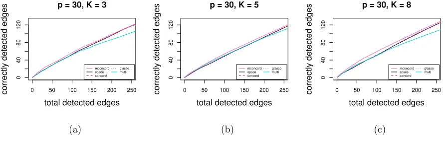
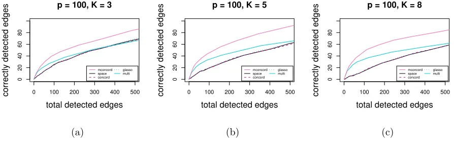
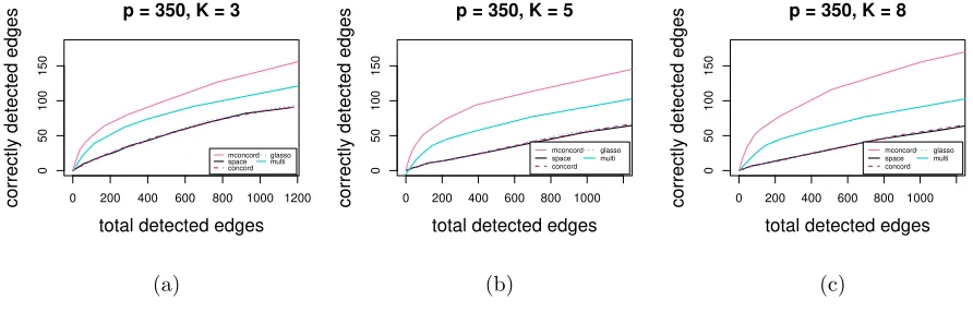
In the first study, we evaluate the performance of each method at a series of different values of the tuning parameter λ. Four random networks with p = 30 (44% density), p = 50 (21% density), p = 100 (6% density), p = 200 (2% density) and p = 350 (2% density) nodes are generated, and each node has a K-dimensional Gaussian variable associate with it, K = 3,5,8. Based on each network, we construct a pK×pK precision matrix, with non-zero blocks corresponding to edges in the network. Elements of diagonal blocks are set as random numbers from [0.5,1]. If nodeiand node j (i < j) are not connected, then the entire (i, j)th and (j, i)th blocks would take values zero. If node i and node j (i < j) are connected, the (i, j)th block would have elements taking values in (0,0.05,−0.05,−0.2,0.2) with equal probabilities so that both strong and weak signals are included. The (j, i)th block can be obtained by symmetry. Finally, we add ρIto the precision matrix to make it positive-definite, whereρis the absolute value of the smallest eigenvalue plus 0.5 and I is the identity matrix. Using each precision matrix, we generate 50 independent datasets consisting of n= 50 (for thep= 30 and p= 50 networks) andn= 100 (for thep= 100,p= 200 andp= 350 networks) i.i.d. samples. Results are given in Figure 1 to Figure 5. All figures show the number of correctly detected edges (Nc) versus the number of total detected edges
0 50 100 150 200 250
Figure 1: Estimation accuracy comparison: total detected edges vs. correctly detected edges with 190 true edges (44%): (a) K= 3; (b) K = 5; (c)K = 8
0 100 200 300 400 500
Figure 3: Estimation accuracy comparison: total detected edges vs. correctly detected edges with 279 true edges (6%): (a)K = 3; (b) K= 5; (c) K = 8
0 200 400 600 800 1000 1200
0
50
100
150
p = 350, K = 3
total detected edges
correctly detected edges
mconcord space concord
glasso multi
(a)
0 200 400 600 800 1000
0
50
100
150
p = 350, K = 5
total detected edges
correctly detected edges
mconcord space concord
glasso multi
(b)
0 200 400 600 800 1000
0
50
100
150
p = 350, K = 8
total detected edges
correctly detected edges
mconcord space concord
glasso multi
(c)
Figure 5: Estimation accuracy comparison: total detected edges vs. correctly detected edges with 1250 true edges (2%): (a)K = 3; (b) K= 5; (c) K = 8
We can observe that for all methods,Nt decreases when we increaseλ. It can be seen thatmconcord
consistently outperforms its counterparts, as it detects more correct edges than the other methods for the same number of total edges detected, especially when we have large K or large p. In all scenarios, space, concord and glassogive very similar results. With largeK and p, multiperforms better than univariate methods.
The better performance of moncord overspace,concord and glasso is largely due to the fact that mconcord is designed for multivariate network, and treating the precision matrix by different blocks is more likely to catch an edge even when the signal is comparably weak. On the contrary, the univariate approaches tend to select more unwanted edges since there is high probability that there is at least on non-zero element in the block due to randomness.
5.2 Model Selection Comparison
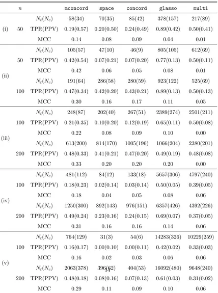
Next in the second study, we compare the model selection performance of the above approaches. We fix K = 4, and conduct simulation studies for several combinations of n and p with different densities which vary from 41% to 1%. The precision matrices are generated using the same technique as in the first study. The tuning parameter λis selected using a 5-fold cross-validation for all methods. We also studied the performance of the Bayesian Information Criterion (BIC) for model selection, but it seems that BIC does not work in the multi dimensional settings. In fact, BIC in most cases tends to choose the smallest model where no edge can be detected. Here we compare sensitivity (TPR), precision (PPV) and Matthew’s Correlation Coefficient (MCC) defined by
TPR = TP
TP + FN,PPV = TP
TP + FP,MCC =
TP×TN−FP×FN p
Table 1: Model selection comparison with p the number of nodes,q the number of true edges and nthe sample size with the tuning parameter λ optimized by cross-validation. Cases considered below are (i) p = 30, q = 177 (41% density) (ii) p= 50, q = 137 (11% density), (iii) p = 100, q = 419 (8% density), (iv) p = 200, q = 617 (3% density), (v)p= 400, q = 782 (1% density) where the density is 100q/ p2 in percentage.
n mconcord space concord glasso multi
(i) 50
Nt(Nc) 58(34) 70(35) 85(42) 378(157) 217(89)
TPR(PPV) 0.19(0.57) 0.20(0.50) 0.24(0.49) 0.89(0.42) 0.50(0.41)
MCC 0.14 0.08 0.09 0.04 0.01
(ii) 50
Nt(Nc) 105(57) 47(10) 46(9) 805(105) 612(69)
TPR(PPV) 0.42(0.54) 0.07(0.21) 0.07(0.20) 0.77(0.13) 0.50(0.11)
MCC 0.42 0.06 0.05 0.08 0.01
100
Nt(Nc) 191(64) 286(58) 280(59) 923(122) 525(69)
TPR(PPV) 0.47(0.34) 0.42(0.20) 0.43(0.21) 0.89(0.13) 0.50(0.13)
MCC 0.30 0.16 0.17 0.11 0.05
(iii) 100
Nt(Nc) 248(87) 202(40) 267(51) 2389(274) 2501(211)
TPR(PPV) 0.21(0.35) 0.10(0.20) 0.12(0.19) 0.65(0.11) 0.50(0.08)
MCC 0.22 0.08 0.09 0.10 0.00
200
Nt(Nc) 613(200) 814(170) 1005(196) 1066(204) 2380(201)
TPR(PPV) 0.48(0.33) 0.41(0.21) 0.47(0.20) 0.49(0.19) 0.48(0.08)
MCC 0.33 0.20 0.20 0.20 0.00
(iv) 100
Nt(Nc) 481(112) 84(12) 133(18) 5657(306) 4797(240)
TPR(PPV) 0.18(0.23) 0.02(0.14) 0.03(0.14) 0.50(0.05) 0.39(0.05)
MCC 0.18 0.04 0.05 0.08 0.06
200
Nt(Nc) 1250(300) 892(143) 976(151) 6357(426) 4392(226)
TPR(PPV) 0.49(0.24) 0.23(0.16) 0.24(0.15) 0.69(0.07) 0.37(0.05)
MCC 0.31 0.16 0.16 0.14 0.06
(v) 100
Nt(Nc) 764(129) 31(3) 54(6) 14283(326) 10229(259)
TPR(PPV) 0.16(0.17) 0.00(0.10) 0.00(0.11) 0.42(0.02) 0.33(0.03)
MCC 0.16 0.02 0.03 0.06 0.06
200
Nt(Nc) 2063(378) 396(62) 404(53) 16092(480) 9648(240)
Table 1 shows that substantial gain is achieved by considering the multivariate aspect in mconcord compared with the univariate methods space and concord in regards of both sensitivity and precision, except for the case p = 30 and n = 50 where these two methods score slightly better TPR due to more selection of edges. Both glasso and multi select very dense models in nearly all cases, and as a consequence their TPR are higher. However, in terms of MCC which accounts for both correct and incorrect selections, mconcordperforms consistently better than all the other methods.
6
Application
6.1 Gene/Protein Network Analysis
According to the NCI website https://dtp.cancer.gov/discovery development/nci-60, “the US National Cancer Institute (NCI) 60 human tumor cell lines screening has greatly served the global cancer research community for more than 20 years. The screening method was developed in the late 1980s as an in vitro drug-discovery tool intended to supplant the use of transplantable animal tumors in anticancer drug screening. It utilizes 60 different human tumor cell lines to identify and characterize novel compounds with growth inhibition or killing of tumor cell lines, representing leukemia, melanoma and cancers of the lung, colon, brain, ovary, breast, prostate, and kidney cancers”.
We apply our method to a dataset from the well-known NCI-60 database, which consists of protein profiles (normalized reverse-phase lysate arrays for 94 antibodies) and gene profiles (normalized RNA microarray intensities from Human Genome U95 Affymetrix chip-set for more than 17000 genes). Our analysis will be restricted to a subset of 94 genes/proteins for which both types of profiles are available. These profiles are available across the same set of 60 cancer cell lines. Each gene-protein combination is represented by its Entrez ID, which is a unique identifier common for a protein and a corresponding gene that encodes this protein.
Three networks are studied: a network based on protein measurements alone, a network based on gene measurements alone, and a gene-protein multivariate network. For protein alone and gene alone networks, we use concord, and for gene-protein network, we use mconcord. The tuning parameter λ is selected using 5-fold cross-validation for all three networks.
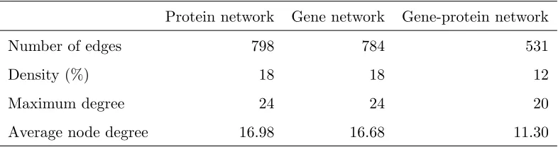
while gene and gene-protein networks share 287 edges. However, protein and gene networks only share 167 edges. Table 2 provides summary statistics for these networks.
Table 2: Summary statistics for protein, gene and gene-protein networks
Protein network Gene network Gene-protein network
Number of edges 798 784 531
Density (%) 18 18 12
Maximum degree 24 24 20
Average node degree 16.98 16.68 11.30
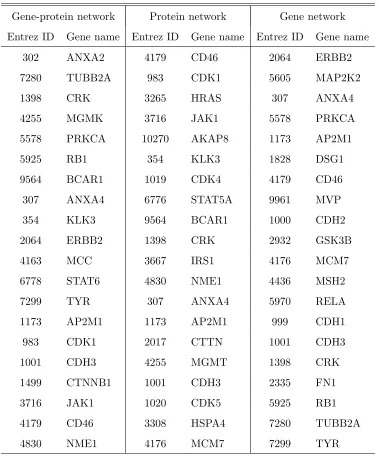
Table 3: Top 20 most connected nodes for three networks (sorted by decreasing degrees)
Gene-protein network Protein network Gene network Entrez ID Gene name Entrez ID Gene name Entrez ID Gene name
302 ANXA2 4179 CD46 2064 ERBB2
7280 TUBB2A 983 CDK1 5605 MAP2K2
1398 CRK 3265 HRAS 307 ANXA4
4255 MGMK 3716 JAK1 5578 PRKCA
5578 PRKCA 10270 AKAP8 1173 AP2M1
5925 RB1 354 KLK3 1828 DSG1
9564 BCAR1 1019 CDK4 4179 CD46
307 ANXA4 6776 STAT5A 9961 MVP
354 KLK3 9564 BCAR1 1000 CDH2
2064 ERBB2 1398 CRK 2932 GSK3B
4163 MCC 3667 IRS1 4176 MCM7
6778 STAT6 4830 NME1 4436 MSH2
7299 TYR 307 ANXA4 5970 RELA
1173 AP2M1 1173 AP2M1 999 CDH1
983 CDK1 2017 CTTN 1001 CDH3
1001 CDH3 4255 MGMT 1398 CRK
1499 CTNNB1 1001 CDH3 2335 FN1
3716 JAK1 1020 CDK5 5925 RB1
4179 CD46 3308 HSPA4 7280 TUBB2A
4830 NME1 4176 MCM7 7299 TYR
6.2 GDP Network Analysis
trade (wholesale), (7) retail trade (retail), (8) transportation and warehousing (trans), (9) information (info), (10) finance and insurance (finance), (11) real estate and rental and leasing (real), (12) profes-sional, scientific and technical services (prof), (13) management of companies and enterprises (manage), (14) administrative and waste management services (admin), (15) educational services (edu), (16) health care and social assistance (health), (17) arts, entertainment and recreation (arts), (18) accommodation and food services (food), (19) other services except government (other) and (20) government (gov).
The data is available from the first quarter of 2005 to the second quarter of 2016. Data from the third quarter of 2008 to the forth quarter of 2009 is eliminated to reduce the impact of the financial crisis of that period. The data is in 8 regions in the US, including New England (Connecticut, Maine, Massachusetts, New Hampshire, Rhode Island and Vermont), Mideast (Delaware, D.C., Maryland, New Jersey, New York and Pennsylvania), Great Lakes (Illinois, Indiana, Michigan, Ohio and Wisconsin), Plains (Iowa, Kansas, Minnesota, Missouri, Nebraska, North Dakota and South Dakota), Souteast (Alabama, Arkansas, Florida, Georgia, Kentucky, Louisiana, Mississippi, North Carolina, South Carolina, Tennessee, Virginia and West Virginia), Southwest (Arizona, New Mexico, Oklahoma and Texas), Rocky Mountain (Colorado, Idaho, Montana, Utah and Wyoming) and Far West (Alaska, California, Hawaii, Nevada, Oregon and Washington).
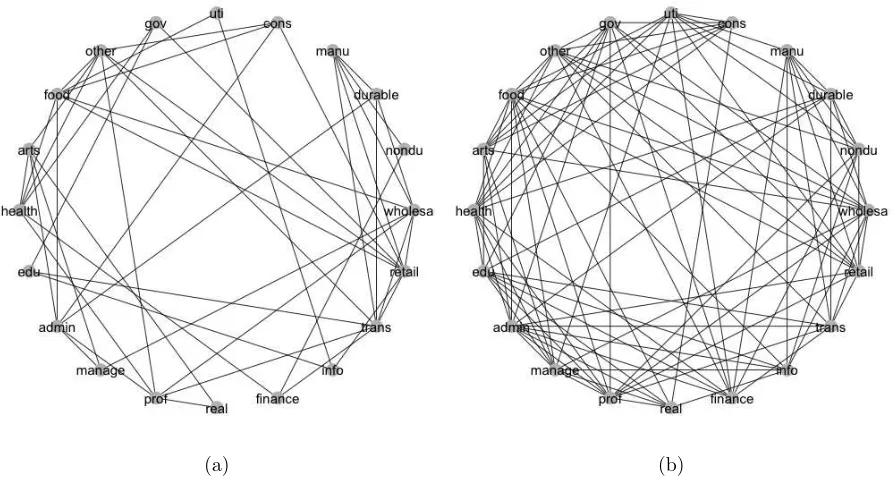
We reduce correlation in the time series data by taking differences of the consecutive observations. A multivariate network consisting of 20 nodes and 8 attributes for each node is studied. After using 5-fold cross-validation to select the tuning parameterλ, 47 edges are detected, with density of 24.7% and average node degree of 4.7. The 5 most connected industries are retail trade, transportation, wholesale trade, accommodation and food services, and professional and technical services. The network is shown in Figure 4(a). It is obvious to see hubs comprising of wholesale trade and retail trade. This is very natural for the consumer-driven economy of the US. Both of these two nodes are connected to transportation, as both of these industries heavily rely on transporting goods. Another noticeable fact is that education is connected with government. As part of the services provided by government, it is natural that the quality as well as GDP of educational services can both be influenced by government.
technical services and health care and social assistance. The network is shown in Figure 4(b). The more modest degree of connections in the multivariate network seems to be more interpretable.
(a) (b)
Figure 6: Comparison of multivariate and univariate GDP networks
7
Proof of the theorems
We rewrite (3) as L(ω, σ,Y) = 1
2 Pp
i=1 PKi
k=1wik
Yik+Pj6=i
PKj
l=1ωijklY˜jl
2
, where ˜Yik =Yik/σik.
For any subset S ⊂ T, the Karush-Kuhn-Tucker (KKT) condition characterizes a solution of the optimization problem
arg min
ω:ωSc=0
Ln(ω,σ, Yˆ ) +λn X
1≤i<j≤p
v u u tXKi
k=1
Kj X
l=1 ω2
ijkl
.
A vector ˆω is a solution if and only if for any (i, j, k, l)∈S
L′n,ijkl(ˆω,σ, Yˆ ) =−λn
ˆ ωijkl
r P
k′,l′
ˆ ω2
ijk′l′
, if∃1≤k≤Ki,1≤l≤Kj,ωˆijkl6= 0
The following lemmas will be needed in the proof of Theorems 1–3. Their proofs are deferred to the Appendix.
Lemma 1 The following properties hold.
(i) For allω and σ,L(ω, σ,Y)≥0.
(ii) If σik>0 for all 1≤k≤Ki and i= 1, . . . , p, then L(·, σ, Y) is convex in ω and is strictly convex
with probability one.
(iii) For every index (i, j, k, l) withi6=j, L¯′
ijkl(¯ω,¯σ) = 0.
(iv) All entries of Σ¯ are bounded and bounded below. Also, there exist constants 0<σ¯0 ≤σ¯∞<∞such
that
¯
σ0≤min{σ¯ik: 1≤i≤p,1≤k≤Ki} ≤max{σ¯ik: 1≤i≤p,1≤k≤Ki} ≤σ¯∞.
(v) There exists constants 0<ΛL
min(¯ω,σ)¯ ≤ΛLmax(¯ω,σ)¯ <∞, such that
0<ΛLmin(¯ω,σ)¯ ≤λmin( ¯L′′(¯ω,σ))¯ ≤λmax( ¯L′′(¯ω,σ))¯ ≤ΛLmax(¯ω,σ)¯ <∞.
Lemma 2 (i) There exists a constant N < ∞, such that for all 1 ≤ i 6= j ≤ p and 1 ≤ k ≤ Ki,
1≤l≤Kj, L¯′′ijkl,ijkl(¯ω,¯σ)≤N.
(ii) There exists constantsM1, M2 <∞, such that for any 1≤i < j≤p,
Var(L′ijkl(¯ω,σ, Y¯ ))≤M1, Var(L′′ijkl,ijkl(¯ω,σ, Y¯ ))≤M2.
(iii) There exists a positive constant g, such that for all (i, j, k, l)∈ A,
L′′ijkl,ijkl(¯ω,σ)¯ −Lijkl,′′ A−ijkl(¯ω,¯σ)hL′′A−ijkl,A−ijkl(¯ω,σ)¯ i−1L′′Aijkl,ijkl(¯ω,σ)¯ ≥g,
where A−ijkl =A \ {(i, j, k, l)}.
(iv) For any (i, j, k, l)∈ Ac, kL¯′′ijkl,A(¯ω,σ)[ ¯¯ L′′A,A(¯ω,σ)]¯ −1k2≤M3.for some constant M3.
Lemma 3 There exists a constantM4 <∞, such that for any1≤i≤j≤pand1≤k≤Ki,1≤l≤Kj,
Lemma 4 Let the conditions of Theorem 2 hold. Then for any sequenceCn→ ∞,
hold with probability tending to 1.
Lemma 5 If Kmax2 qn =o(
p
n/logn), then for any sequence Cn → ∞ and any u ∈ R|A|, the following
hold with probability tending to 1:
kL′n,A(¯ω,σ,ˆ Y)k2 ≤ CnKmax
Lemma 6 Assume that the conditions of Theorem 1 hold. Then exists a constant C¯1 > 0, such that
with probability tending to 1, there exists a local minimum of the restricted problem (4) within the disc
{ω:kω−ω¯k2 ≤C¯1Kmax√qnλn}.
Lemma 7 Assume the conditions of Theorem 1. Then exists a constant C¯2 > 0 such that for any
ω satisfying kω −ω¯k2 ≥ C2Kmax¯ √qnλn and ωAc = 0, we have kL′
n,A(ω,σ,ˆ Y)k2 > Kmax√qnλn with
probability tending to 1.
Lemma 8 LetDA,A(¯ω,σ, Y¯ ) =L′′A,A(ω,σ, Y¯ )−L¯′′A,A(¯ω,¯σ). Then there exists a constant M5 <∞, such
that for any (i, j, k, l)∈ A,λmax(Var(DA,ijkl(¯ω,σ, Y¯ )))≤M5.
Proof 1 (of Theorem 1) The existence of a solution of (4) follows from Lemma 6. By the KKT
o(λn), by virtue of the assumption thatλn
p
n/logn→ ∞.
Note that by Theorem 1,kνnk2 ≤CnKmax√qnλn with probability tending to 1. Thus as in Lemma 5, for
sufficiently slowly growing sequenceCn→ ∞,|Dn,ijkl,A(¯ω,ˆσ,Y)νn| ≤CnKmax p
qn(logn)/nKmax√qnλn=
o(λn) with probability tending to 1. This claim follows from the assumptionKmax2 qn=o(
p
n/logn). Finally, let bT = ¯L′′ijkl,A(¯ω,σ)[ ¯¯ L′′A,A(¯ω,¯σ)]−1. By the Cauchy-Schwartz inequality
|bTDn,A,A(¯ω,σ,¯ Y)νn| ≤ kbTDn,A,A(¯ω,σ,¯ Y)k2kνnk2
≤ Kmax2 qnλn max
(i′,j′,k′,l′)∈A|b TD
n,A,i′j′k′l′(¯ω,σ,¯ Y)|.
In order to show that the right hand side is o(λn) with probability tending to 1, it suffices to show
max (i′,j′,k′,′l)∈A|b
TD
n,A,i′j′k′l′(¯ω,σ,¯ Y)|=O
r logn
n !
with probability tending to 1, because of the assumption Kmax2 qn = o(
p
n/logn). This is implied by E(|bTDA,i′j′k′l′(¯ω,σ, Y¯ )|2) ≤ kbk2
2λmax(Var(DA,i′j′k′l′(¯ω,σ, Y¯ ))) being bounded, which follows
immedi-ately from Lemma 1(iv) and Lemma 8. Finally, as in Lemma 5,
|bTDn,A,A(¯ω,ˆσ,Y)νn| ≤ |bTDn,A,A(¯ω,σ,¯ Y)νn|
+|bT(Dn,A,A(¯ω,σ,¯ Y)−Dn,A,A(¯ω,σ,ˆ Y))νn|,
where by Lemma 4, the second term on the right hand side is bounded by Op(
p
(logn)/n)kbk2kνnk2. Note that kbk2 =O(Kmax√qn), thus the second term is also of ordero(λn) by the assumptionKmax2 qn=
o(pn/logn).
Proof 3 (of Theorem 3) By Theorems 1 and 2 and the KKT condition, with probability tending to 1,
a solution of the restricted problem is also a solution of the original problem. This shows the existence of the desired solution. For part (ii), the assumed condition on the signal strength implies that missing a signal costs more than the estimation error in part (i), and hense it will be impossible to miss such a signal. This shows the selection consistency. If the objective function is strictly convex, the solution is also unique, so this will be the only solution for the original problem.
Finally, convergence properties of the estimator of σ claimed in Proposition 1 is shown.
Proof 4 (of Proposition 1) Observe that when
p
P
i=1
Ki < βn, eik can be expressed as eik = Yik −
YT
−ik(Y−TikY−ik)−1Y−ikYik. As argued in Peng et al. [6], E(eTikeik) = 1/¯σik. Therefore, by Lemma 9 of
the Appendix and Lemma 1(iv), we have max{|σˆik−σ¯ik|: 1≤k≤Ki,1≤i≤p}=Op(
p
Acknowledgement
This research is partially supported by National Science Foundation grant DMS-1510238.
Appendix A. Proof of the lemmas
Proof 5 (of Lemma 1) The assertions (i) and (ii) are self-evident from the definition of L. To prove
(iii), denote the residual for the ith term by eik(ω, σ) = Yik + P
Since all eigenvalues of ¯Σ lie between two positive numbers, so do all diagonal entries because these are val-ues of quadratic forms for unit vectors having 1 at one place. All off-diagonal entries lie in [−Λmax,Λmax] because these are values of bilinear forms at such unit vectors. This shows (iv).
since ¯L′′(¯ω,σ) = E ˜¯ YY˜T, we have
aTL¯′′(¯ω,σ)a¯ =
p
X
i=1
Ki X
k=1
wikaTikΣa˜ ik ≥ p
X
i=1
Ki X
k=1
wikλmin( ˜Σ)kaikk22 ≥2w0λmin( ˜Σ),
where ˜Σ = var( ˜Y). Similarly,aTL¯′′(¯ω)a≤2w
∞λmax( ˜Σ). By Condition C1, ˜Σ has bounded eigenvalues, and hence (v) follows.
Proof 6 (of Lemma 2) The proof of (i) follows because ¯L′′
ijkl,i′j′k′l′(¯ω,σ) =¯ σjl,j′l′ +σik,i′k′, and the
entries of ¯Σ are bounded by Lemma 1(iv).
For (ii) note that Var(eik(¯ω,σ)) = 1/¯¯ σik and Var(Yik) = ¯σik,ik,
Var(L′n,ijkl(¯ω,σ, Y¯ )) = Var(wikeik(¯ω,¯σ)Yjl) + Var(wjlejl(¯ω,σ)Y¯ ik)
≤E(wik2e2ik(¯ω,σ)Y¯ jl2) + E(wjl2e2jl(¯ω,σ)Y¯ ik2) = w 2
ikσ¯jl,jl
¯ σik +
wjl2σ¯ik,ik
¯ σjl .
The right hand side is bounded because of Condition C0 and Lemma 1(iv), and the fact that eik(¯ω,σ)¯
and Yjl are independent.
For (i, j, k, l)∈ A, denote
D:= ¯L′′ijkl,ijkl(¯ω,¯σ)−L¯′′ijkl,A−ijkl(¯ω,σ)¯ hL¯′′A−ijkl,A−ijkl(¯ω,¯σ)i−1L¯′′A−ijkl,ijkl(¯ω,σ).¯
Then D−1 is the (ijkl, ijkl)th entry in hL¯′′
A,A(¯ω,¯σ)
i−1
. Thus by Lemma 1(v), D−1 is positive and bounded from above, so Dis bounded away from zero. This proves (iii).
Note thatkL¯′′
ijkl,A(¯ω,¯σ)[ ¯L′′A,A(¯ω,¯σ)]−1k22≤ kL¯ijkl,′′ A(¯ω,σ)¯ k22λmax([ ¯L′′A,A(¯ω,σ)]¯ −2).By Lemma 1(iv), λmax([ ¯L′′A,A(¯ω,σ)]¯ −2) is bounded from above, thus it suffices to show that kL¯′′ijkl,A(¯ω,σ)¯ k22 is bounded. Define A+ := (i, j, k, l)∪ A. Then ¯L′′
ijkl,ijkl(¯ω,σ)¯ −L¯′′ijkl,A(¯ω,σ)[ ¯¯ LA′′,A(¯ω,σ)]¯ −1L¯′′A,ijkl(¯ω,σ) is the inverse¯
of the (kl, kl) entry of ¯L′′A+,A+(¯ω,σ). Thus by Lemma 1(iv), it is bounded away from zero. Therefore by¯ Lemma 2(i), ¯L′′
ijkl,A(¯ω,σ)[ ¯¯ L′′A,A(¯ω,σ)]¯ −1L¯′′A,ijk(¯ω,σ) is bounded from above. Since¯
¯
L′′ijkl,A(¯ω,¯σ)[ ¯L′′A,A(¯ω,σ)]¯ −1L¯′′A,ijk(¯ω,σ)¯ ≥ kL¯′′ijkl,A(¯ω,σ)¯ k22λmin([ ¯L′′A,A(¯ω,σ)]¯ −1),
and by Lemma 1(iv), λmin([ ¯L′′A,A(¯ω,σ)]¯ −1) is bounded away from zero, we havekL¯′′ijkl,A(¯ω,σ)¯ k22 bounded from above. Thus (iv) follows.
Proof 7 (of Lemma 3) The (i′k′, j′l′)th entry of the matrix Y
ikYjlY˜Y˜T is YikYjlY˜i′k′Y˜j′l′, for 1≤ i <
is E[YikYjlY˜i′k′Y˜j′l′] = (¯σik,jlσ¯i′k′,j′l′ + ¯σik,i′k′σ¯jl,j′l′ + ¯σik,j′l′σ¯jl,i′k′)/(¯σi
covariance between Yik andYjl. Thus, we can write
E[YikYjlY˜Y˜T] = From this, it follows that
kσ¯ik,·k2=kΣ¯−1/(2ik)Σ¯−−1(ik/2)σ¯ik,·k2≤ kΣ¯1−/(2ik)kkΣ¯−−1(ik/2)σ¯ik,·k ≤
Op(1), and hence by Lemma 1(iv) and Condition C3 it follows that
Proof 9 (of Lemma 5) If we replace ˆσ by ¯σon the left hand side and take (i, j, k, l)∈ A, then from the definition we have L′n,ijkl(¯ω,σ,¯ Y) =eik(¯ω,σ)¯ TYjl+ejl(¯ω,σ)¯ TYik, and Yjl, where eik aren replications
of eik( ¯ω,σ). Thus by Lemma 10 of the Appendix we obtain max¯ {|Ln,ijkl′ (¯ω,σ,ˆ Y)| : (i, j, k, l)∈ A} ≤
Cn
p
(logn)/n.and hence by the Cauchy-Schwartz inequality
kL′n,A(¯ω,σ,ˆ Y)k2≤Kmax√qn max right hand side has order Kmax
p
qn(logn)/n. Since there are Kmax2 qn terms and by Lemma 4, they are
uniformly bounded by p(logn)/n. The rest of the lemma can be proved by similar arguments.
Proof 10 (of Lemma 6) Let αn = Kmax√qnλn, and Ln(ω,σ,ˆ Y) = Ln(ω,σ,ˆ Y) +λP Pi<jkωijk2.
Then for any given constant ¯C1 > 0 and any vector u such that uAc = 0 and kuk2 = ¯C1, the triangle inequality and the Cauchy-Schwartz inequality together imply that
X
Thus for any sequence Cn→ ∞, with probability tending to 1,
Ln(¯ω+αnu,σ,ˆ Y)−Ln(¯ω,σ,ˆ Y)
By the assumptions thatK2
maxqn=o(
p
n/logn) andλn
p
n/logn→ ∞, we haveα2
nKmax2 qnn−1/2√logn=
o(α2n) andαnKmaxq1n/2n−1/2√logn=o(α2n). Thus,
Ln(¯ω+αnu,σ,ˆ Y, λn)− Ln(¯ω,σ,ˆ Y, λn)≥
1 4α
2
nuTAL¯′′A,A(¯ω,σ)u¯ A−C¯1α2n
with probability tending to 1. By Lemma 1 (iv), uTAL¯′′A,AuA ≥ΛLmin(¯ω,σ)¯ kuAk22 = ΛminL (¯ω,σ) ¯¯ C12, thus if we take ¯C1= 5/ΛLmin(¯ω,¯σ), then
Pinf{Ln(¯ω+αnu,σ,ˆ Y, λn) :u:uAc = 0,kuk2 = ¯C1}>Ln(¯ω,σ,ˆ Y, λn)→1.
Hence a local minimum exists in {ω:kω−ωˆk2 ≤C¯1Kmax√qnλn}with probability tending to 1.
Proof 11 (of Lemma 7) Letαn=Kmax√qnλn. Anyω in the statement of the lemma can be written
asω = ¯ω+αnu, withuAc = 0 and kuk2 ≥C¯2, where ¯C2 >0. Note that
L′n,A(ω,σ,ˆ Y) =L′
n,A(¯ω,σ,ˆ Y) +αnL′′n,A,A(¯ω,σ,ˆ Y)u
=L′n,A(¯ω,σ,ˆ Y) +αn
L′′n,A,A(¯ω,ˆσ,Y)−L¯′′
A,A(¯ω,¯σ)
u+αnL¯′′A,A(¯ω,σ)u.¯
By the triangle inequality and Lemma 5, for any Cn→ ∞,kL′n,A(ω,σ,ˆ Y)k2 is bounded below by
αnkL¯′′A,A(¯ω,σ)u¯ k2−Cn(Kmaxq1n/2n−1/2
p
logn)−Cnkuk2(αnKmax2 qnn−1/2
p logn)
with probability tending to 1. Thus, as argued in the proof of Lemma 6,αnKmaxqn1/2n−1/2√logn=o(αn)
and αnKmax2 qnn−1/2√logn=o(αn), thenkL′n,A(ω,σ,ˆ Y)k2 ≥ 12αnkL¯′′A,A(¯ω,σ)u¯ k2 with probability tend-ing to 1. By Lemma 1(iv),kL¯′′A,A(¯ω,¯σ)uk2 ≥ΛminL (¯ω,σ)¯ kuk2. Therefore ¯C2can be taken as 3/ΛLmin(¯ω,σ).¯
Proof 12 (of Lemma 8) Observe that Var(DA,ijkl(¯ω,σ, Y¯ )) = E(L′′A,ijkl(¯ω,σ, Y¯ )L′′A,ijkl(¯ω,σ, Y¯ )T) −
¯ L′′
A,ijkl(¯ω,σ) ¯¯ L′′A,ijkl(¯ω,σ)¯ T.Thus it suffices to show that there exists a constantM5>0, such that for all
(i, j, k, l), λmax(E(L′′A,ijkl(¯ω,¯σ, Y)LA′′,ijkl(¯ω,σ, Y¯ )T))≤M5.We use the same notations as in the proof of Lemma 1(v).
Note that L′′A,ijkl(¯ω,σ, Y¯ ) = ˜XTX˜(ik,jl) = YikXjl+YjlXik. Thus E(L′′A,ijkl(¯ω,σ, Y¯ )L′′A,ijkl(¯ω,σ, Y¯ )T) is
given by E[Y2
ikXjlXjlT] + E[Yjl2XikXikT] + E[YikYjl(XjlXjlT +XikXikT)],and for a∈Rd,
aTEω,¯σ¯(L′′A,ijkl(¯ω,σ, Y¯ )L′′A,ijkl(¯ω,σ, Y¯ )Ta = aTjlE[Yik2Y˜Y˜T]ajl+aTikE[Yjl2Y˜Y˜T]aik + 2aTikE[YikYjlY˜Y˜T]ajl.
Since Ppi=1PKi
Appendix B. Auxiliary results
Lemma 9 Let Xij ∼N(0, σi2), i= 1, . . . , m and j = 1, . . . , n. For each i, Xi1, . . . , Xin are assumed to
be i.i.d., but are arbitrarily dependent across i. Then for any sequence Cn→ ∞, with probability tending
to 1, we have max1≤i≤m|n−1Pnj=1Xij2 −σ2i| ≤Cn
p
(logm)/n.
Proof 13 Let Zij =Xij/σi, then for fixed iandr = 2,3, . . ., we have
E|n−1(Zi21−1)|r ≤ 2
r−1
nr E(Z
2r
i1 + 1)≤(2/n)rr! = (2/n)r−2 4 n2r!.
By Lemma 2.2.11 of Van Der Vaart & Wellner [9], taking M = 2/n and v = 8/n, it follows that P|n−1Pnj=1Zij2 −1|> x≤2e−x2/[2(8/n+2x/n)]. Since σi are bounded, Lemma 2.2.10 of Van Der Vaart
& Wellner [9] implies that for some C > 0, Emax1≤i≤m|n−1Pnj=1Xij2 −σ2i|
≤ Cp(logm)/n, which implies the conclusion.
Lemma 10 Let Xij i.i.d.∼ N(0, σ2xi) and Yij i.i.d.∼ N(0, σ2yi) for i= 1, . . . , m and j = 1, . . . , n, and Xij and
Yij are independent for alli. Further assume that0< σxi, σyi ≤σ <∞. Then for any sequenceCn→ ∞,
we have max1≤i≤m|n−1Pnj=1XijYij| ≤Cn
p
(logm)/n.
Proof 14 For fixed iwe can observe that
E|n−1Xi1Yi1|r= 1
nrE|Xi1| rE|Y
i1|r≤ 2rσr
nr
(Γ(r+12 ))2
π ≤(2σ/n)
r−24σ2 πn2r!.
By Lemma 2.2.11 of Van Der Vaart & Wellner [9], taking M = 2σ/n and v = 8σ2/πn, we have P|n−1Pnj=1XijYij|> x
≤2e−x2/[2(8σ2/πn+2σx/n)].Then by Lemma 2.2.10 of Van Der Vaart & Wellner [9], for some C >0, Emax
1≤i≤m|n −1Pn
j=1XijYij|
≤Cp(logm)/n, which implies the conclusion.
References
[1] Onureena Banerjee, Laurent El Ghaoui, and Alexandre dAspremont. Model selection through sparse maximum likelihood estimation for multivariate gaussian or binary data. Journal of Machine Learn-ing Research, 9(Mar):485–516, 2008.
[3] Kshitij Khare, Sang-Yun Oh, and Bala Rajaratnam. A convex pseudolikelihood framework for high dimensional partial correlation estimation with convergence guarantees. Journal of the Royal Statistical Society: Series B (Statistical Methodology), 77(4):803–825, 2015.
[4] Mladen Kolar, Han Liu, and Eric P Xing. Graph estimation from multi-attribute data. Journal of Machine Learning Research, 15(1):1713–1750, 2014.
[5] Nicolai Meinshausen and Peter B¨uhlmann. High-dimensional graphs and variable selection with the lasso. The Annals of Statistics, 34:1436–1462, 2006.
[6] Jie Peng, Pei Wang, Nengfeng Zhou, and Ji Zhu. Partial correlation estimation by joint sparse regression models. Journal of the American Statistical Association, 486:735–746, 2009.
[7] Adam J Rothman, Peter J Bickel, Elizaveta Levina, and Ji Zhu. Sparse permutation invariant covariance estimation. Electronic Journal of Statistics, 2:494–515, 2008.
[8] Paul Tseng. Convergence of a block coordinate descent method for nondifferentiable minimization.
Journal of Optimization Theory and Applications, 109(3):475–494, 2001.
[9] Aad W Van Der Vaart and Jon A Wellner. Weak Convergence and Empirical Processes. Springer, 1996.