IN SITU DETERMINATION OF LAYER THICKNESS
Abdul Ghani Rafek***, & Khairul Anuar Mohd Nayan**** method for determining the stiffness profile of soil and pavement sites. The method consists of generation, measurement, and processing of dispersive elastic waves in layered systems. The test is performed on the pavement surface at strain level below 0.001%, where the elastic properties are considered independent of strain amplitude. During an SASW test, the surface of the medium under investigation is subject to an impact to generate energy at various frequencies. Two vertical acceleration transducers are set up near the impact source to detect the energy transmitted through the testing media. By recording signals in digitised form using a data acquisition system and processing them, surface wave velocities can be determined by constructing a dispersion curve. Through forward modeling, the shear wave velocities can be obtained, which can be related to the variation of stiffness with depth. This paper presents the results of two case studies for near-surface profiling of two different asphalt pavement sites.
INTRODUCTION
There are more than 60,000 kilometers of expressways and roads in Malaysia, of which more than one half are either flexible or rigid pavements. The serviceable period for flexible pavement is approximately 20 years, whereas rigid pavements may achieve a longer serviceable period of more than 50 years. Most of the expressways, federal roads, state roads and council roads are more than 20 years old. Owing to aging roads and increasing traffic loads and volumes, the responsibility for maintenance, rehabilitation and management of pavement structures is becoming more and more critical. Therefore, the need for accurate, fast, cost effective and non-destructive evaluation of the pavement structure is becoming ever more important. Periodic evaluation is being done to fulfill the requirement for QA/QC purposes, but more importantly to detect symptoms of deterioration at early stages for their economic management.
Soil, rock-fill, bitumen and concrete material used in pavement structures usually behave non-linearly under the loads of passing heavy vehicles. However, at lower stress level (0.001%), they are nearly linear and can propagate elastic waves. Recent advancement and improvement of the well-known steady-state Rayleigh wave method (Richart et al. 1970) resulted in a promising new NDT method known as the spectral analysis of surface waves (SASW) method (Heisey et al. 1982; Nazarian & Stokoe 1984). The SASW technique successfully reduces the field-testing time and improves the accuracy of the original steady-state method. It also overcomes many of the limitations of the well-known deflection-basin-based method, e.g., the falling weight deflectometer or dynaflect.
The purpose of this paper is to describe the role of the SASW technique in assisting pavement engineers in evaluation and management of highways. The first part of the paper discusses the fundamentals of the SASW method and properties of pavement that can be detected by the method. The second section illustrates the results of the SASW tests in pavement investigations.
RESEARCH METHODOLOGY
Propagation of Rayleigh Waves
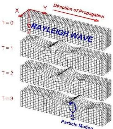
Figure 1. The particle motion and direction of Rayleigh propagation in a homogeneous, elastic and isotropic medium
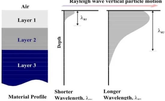
In homogenous, isotropic, elastic half-space, Rayleigh wave velocity does not vary with frequency. However, in the layered medium where there is a variation of stiffness with depth, Rayleigh wave velocity is frequency dependent. This phenomenon is termed dispersion where Rayleigh wave refers to the variation of phase velocity as a function of wavelength. The ability for detecting and evaluating the depth of the medium is influenced by the wavelength and the frequency generated. Fig. 2 shows that the shorter wavelength of higher frequency penetrates the shallow zone of the near surface and the longer wavelength of the lower frequency penetrates deeper into the medium.
Rayleigh wave propagation technique may be used to determine the parameters of the elastic moduli of pavement and soil layers. These parameters represent the material behaviour at small shearing strain, of less than of 0.001 % [20]. In this strain range, material behaviour, particularly the sub grade material, is typically independent of strain amplitude. Nazarian and Stokoe [17] explained that the elastic moduli of material are constant below a strain of about 0.001 % and is equal to Emax and its corresponding Gmax.
E =
2
V
s2g
(1 + µ) (1)where, E = dynamic Young’s modulus, Vs = shear wave velocity, γ = total unit
weight of the pavement or soil, g = gravitational acceleration, and µ = Poisson’s ratio.
Figure 2. Variation of vertical particle motion for Rayleigh waves with different wavelengths.
Field Procedure
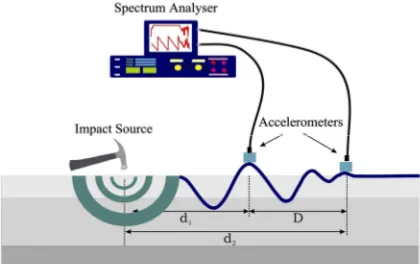
A schematic of the SASW test is shown in Fig. 3. Elastic waves are generated (by means of impacts), on the surface of pavement and are detected by a pair or an array of receivers. A portable 4-channel dynamic spectrum analyser (OROS OR25 PC-Pack II) was utilized for recording and analysing the data. The common receiver midpoint (CRMP) array geometry was used (see Nazarian 1984 for detail). The spacing between receivers was 0.1, 0.2, 0.4, 0.8, 1.6, and 3.2 m. Piezoelectric accelerometers were used to pick up the surface wave signal. The accelerometers were glued to the pavement surface to ensure good coupling. The dynamic signal is generated in the pavement using a variety of impact sources depending on the frequency range of interest, which in turn influence the sampling depth. For small spacings, steel ball bearings, which tend to produce signal with substantial high frequency to sample shallow layers were used. On the other hand, hammers were employed for larger spacings to produce low frequency signals to sample deeper layers.
Nazarian and Stokoe (1985) suggested an average of five signals was considered adequate. The outputs in the time domain were transformed through a Fast Fourier Transform (FFT) to X(t) and Y(t) in the frequency domain by the analyser.
Two functions in the frequency domain (i.e. the phase spectrum and coherence function) were utilized for analysing the averaged data signals. The
cross power spectrum, GXY, between the two receivers is defined as
f Y f XGXY *. (2)
where X
f * denotes the complex conjugate of X
f . The phase shift, XY
f , which represents physically the number of cycles that each frequency possesses in distance D between the two receivers, can be computed as
Y
XY XY
X
XY f f tan ImG ReG
1
(3) where XY
f is the phase shift of the cross power spectrum at each frequency,
GXYIm and Re
GXY are the imaginary and real parts of the cross power spectrum at each frequency, and f is the frequency in cycles per seconds (or Hz).Figure 3. Layout of the testing set-up of the SASW method for pavement
evaluation.
The coherence function is the ratio of the output power caused by the measured input to the total measured output. If some noise is generated in the system, the coherence is less than one since the total measured output includes not only the output power due to the measured input but also noise output due to the input noise and noise at the output side. The coherence function, 2
f , is mathematically defined as :
f GXY
GXX.GYY
2 2
Where,GXX X
f .X f is the power spectrum of first receiver, and
f Y fY
GYY . is the power spectrum of second receiver. The value of coherence function in the range of frequencies being measured is between zero and one and is a good tool for assessing the quality of the observed signals. A value of criterion for accepting data in pavement evaluation. Sayyedsadr & Drnevich (1989), however, used a default value of 0.98 as a minimum coherence magnitude. In this study, the acceptance of data is set at a coherence magnitude of at least 0.95. If this criterion was not satisfied, the test data was excluded and the test was repeated using different sources or impact surfaces, e.g. employing rubber pads, until satisfactory data were obtained. In most cases coherence magnitudes above 0.98 were obtained over the frequency range of interest.
Construction of Dispersion Curve
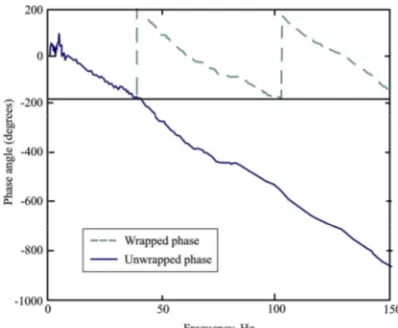
When displaying the phase spectra, the analyser may not use full-scale display, instead it may display the phase in the range of ±180º and hence cause it to wrap. The step to find the actual phase of a frequency is to count the number of full 360º cycles preceding the frequency and to add that to the fraction of the last cycle or the frequency (Fig. 4). The process is called unwrapping of the phase (Nazarian 1984). Data points that did not satisfy the following two criteria were discarded: (i) a coherence magnitude of 0.95, and (ii) a wavelength greater than ½D and less than 3D (Heisey et al. 1982). This operation is called ‘masking’.
By repeating the procedure outlined by Eq. (6) through (8) for every frequency, the Rayleigh wave velocity corresponding to each wavelength is evaluated and the experimental dispersion curve is generated. It should be noted that velocities obtained from an experimental dispersion curve are not the actual Rayleigh wave velocities, but rather apparent or phase velocities. The existence of layers with higher or lower velocities at the surface of a medium, such as a pavement structure, affects the measurement of the velocities of the underlying layers. Thus, a method for evaluating the actual Rayleigh wave velocities from apparent Rayleigh wave velocities is necessary in the SASW test.
Figure 4. Wrapped and unwrapped phase spectra.
ANALYSIS AND DISCUSSION
Inversion of Dispersion Curve
The process of converting the dispersion curve into the shear wave velocity profile is called inversion or forward modeling. Data points of the experimental dispersion curve are usually compressed into a smaller number of data points by averaging a certain range of experimental data points into one data point. There are basically two inversion processes, a simple and a refined one.
The simple inversion process is based on an earlier inversion of the steady-state vibration technique (Richart et al. 1970). The inversion is done by assigning the shear wave velocity equal to 1.1 times the phase velocity and the depth is 0.33 times the wavelength. It provides satisfactory results for geotechnical sites where the shear modulus smoothly increases with depth (Matthews et al. 1996). However, in cases where there is a large contrast in shear wave velocities, such as in pavement systems, this simple method can lead to erroneous results.
available for SASW applications. Among them are: (1) the transfer matrix method (Haskell, 1953; Thomson, 1950); (2) the dynamic stiffness matrix method (Kausel & Röesset, 1981); and (3) the finite difference method (Hossain & Drnevich, 1989). The transfer and stiffness matrix methods provide exact formulation as compared to the other methods (Ganji et al. 1998). Although the approach of the inversion methods can be different, however, all the methods assume that the profile consists of a set of homogeneous layers extending to infinity in the horizontal direction. The last layer is usually considered as a homogeneous half-space.
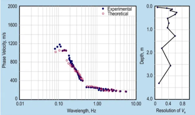
Figure 5. Comparison between averaged experimental theoretical dispersion curve and resolution of shear wave velocity at SASW array PREC11-JP1.
Calculation of the Elastic Moduli
According to elastic theory, the velocity of shear wave, VS, is related to the velocity of Rayleigh wave propagation, VR, by
R
S CV
V (8)
where C is a function of Poisson’s ratio, and C
1.1350.182
for 0.1. Misjudging has little effect on VS(Nazarian et al. 1983). The shear modulus, G, is related to the shear wave velocity by2
S
V g
G (9)
and the Young’s modulus, E, is related to G by
2G1E (10)
CASE STUDY 1: LANDED-ZONE 4-B, PRECINT 11, PUTRAJAYA
The SASW testing was carried out on a pavement surface at Landed-Zone 4-B, Precint 11, Putrajaya construction project (SASW array PREC11-JP1). The pavement profile consists of an asphalt layer (100 mm thick), a base of crushed aggregates (300 mm thick), and a sub base of sand (200 mm thick) over a metasediment sub grade. Material properties and thickness of the four layers are shown in Figure 6(a). In this study, the receiver spacing of 10, 20, 40, 80, 160 and 320 cm were used. of the base followed by a gradual increase of the modulus for the sub base and sub grade with elastic modulus of around 10 MPa.
CASE STUDY 2: KM 296, NORTH – SOUTH EXPRESSWAY
The SASW testing was carried out on a pavement surface at Km 296 (North Bound), Seremban – Bangi section of the North – South Expressway (SASW array LRSB-ApJ) during rehabilitation works. The pavement structure consists of an asphalt layer (180 - 200 mm thick), a sub base of crushed aggregates and fine sand (2000 - 2500 mm thick), over a metasediment sub grade. Material properties and thickness of the four layers are shown in Figure 7(a). In this study, the receiver spacing of 10, 25, 50, 100, and 200 cm were used. The sources for the Rayleigh wave employed were slightly different from those in the case study 1. For high frequency signals, 2-inch nail and small hammers were used, while geological hammer was used for receiver spacing higher than 100 cm.
(a) (b) (c)
Figure 6. (a) The designed pavement profile, (b) the final shear wave profile from the inversion analysis, and (c) the calculated dynamic Young
modulus profile at SASW array PREC11-JP1.
(a) (b) (c)
Figure 7. (a) The pavement structure profile, (b) The final shear wave profile from the inversion analysis, and (c) the calculated dynamic Young modulus profile at
CONCLUDING REMARKS
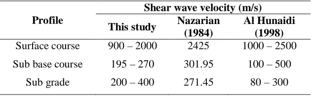
Samples of the asphalt pavement structure for laboratory analysis were not available during the study. The thickness of layering obtained from the inversion analysis compared well with the existing profile obtained from the construction record. The shear wave velocities and dynamic Young’s modulus profiles from this study were compared with SASW testing that had been carried out by other workers, such as Nazarian (1984) and Al Hunaidi (1998) (Table 1). In general, there is a reasonable agreement between the results from this study and their results.
Table 1. Comparison of shear wave velocity from this study to that of Nazarian (1984) and Al-Hunaidi (1998). with reasonable accuracy, unlike the drawbacks from the other seismic methods for this case.
REFERENCES
Al-Hunaidi, M.O. 1998. Evaluation-based genetic algorithms for analysis of non-destructive surface waves test on pavements, NDT &E International, Vol.31, No.4, pp.273-280.
Ganji, V., Gucunski, N & Nazarian, S. 1998. Automated Inversion Procedure For Spectral Analysis of Surface Wave. Journal of Geotechnical and Geoenvironmental Engineering, August 1998, pp.757-770.
Haskell, N.A. 1953. The Dispersion of surface waves in multi-layered media. Bull. Seismol. Soc. Am., Vol. 43, No. 1, pp 17-34.
Bush, A.J., III & Baladi, G.Y. American Society for Testing and Materials, Special Technical Publication 1026, pp. 649-669.
Heisey, J.S., Stokoe II, K.H. & Meyer, A.H., 1982. Moduli of pavement systems from Spectral Analysis of Surface Waves. In Transportation Research Record 852, TRB, National Research Council, Washington, D.C., pp 22-31. Heisey, J.S., 1982, Determination of In Situ Shear Wave Velocity from Spectral
Analysis of Surface Wave. Master Thesis, University of Texas, Austin, pp.300.
Joh, S.-H., 1996. Advances in data interpretation technique for Spectral Analysis-of-Surface-Waves (SASW) measurements. Ph.D. Dissertation, the University of Texas at Austin, Austin, Texas, U.S.A., 240 pp.
Kausel, E. & Röesset, J.M., 1981. Stiffness matrices for layered soils. Bull. Seismol. Soc. Am., 72, pp 1743-1761.
Matthews, M.C., Hope, V.S. & Clayton, R.I., 1996. The geotechnical value of ground stiffness determined using seismic methods. In Proc. 30th Annual Conf. of the Eng. Group of the Geol. Soc., University of Lige, Belgium. Nazarian, S., 1984. In-situ determination of elastic moduli of soil deposits and
pavement systems by Spectral-Analysis-Of-Surface-Wave Method. Ph.D. Dissertation, University of Texas at Austin, 452 pp.
Nazarian, S. & Stokoe II, K. H. 1984. In-situ shear wave velocity from spectral analysis of surface waves. Proc. 8th World Conf. On Earthquake Engineering, 3, pp 31-38.
Richart, F.E.Jr., Hall, J.R., Jr. & Woods, R.D. 1970. Vibrations of soils and foundations. New Jersey: Prentice-Hall.
Sayyedsadr, M. & Drnevich, V.P. 1989. SASWOPR: A program to operate on spectral analysis of surface wave data. In Non-destructive testing of pavements and back-calculation of moduli. Edited by A.J. Bush III & G.Y. Baladi. American Society for Testing and Materials, Special Technical Publication 1026, pp 670-682
Stokoe II, K.H., Wright, S.G., Bay, J.A. & Röesset, J.M., 1994. Characterization of geotechnical sites by SASW method. Geotechnical characterization of sites, R.D. Wood (Ed), Oxford and IBH Publishing Co., New Delhi, India, 15-26. Thomson, W.T. 1950. Transmission of elastic waves through a stratified solid