Full Terms & Conditions of access and use can be found at
http://www.tandfonline.com/action/journalInformation?journalCode=ubes20
Download by: [Universitas Maritim Raja Ali Haji] Date: 12 January 2016, At: 23:28
Journal of Business & Economic Statistics
ISSN: 0735-0015 (Print) 1537-2707 (Online) Journal homepage: http://www.tandfonline.com/loi/ubes20
Comment
Eric Ghysels & Arthur Sinko
To cite this article: Eric Ghysels & Arthur Sinko (2006) Comment, Journal of Business & Economic Statistics, 24:2, 192-194, DOI: 10.1198/073500106000000080
To link to this article: http://dx.doi.org/10.1198/073500106000000080
Published online: 01 Jan 2012.
Submit your article to this journal
Article views: 45
View related articles
192 Journal of Business & Economic Statistics, April 2006
Bandi, F., and Russell, J. (2005a), “Microstructure Noise, Realized Volatility, and Optimal Sampling,” working paper, University of Chicago, Graduate School of Business.
(2005b), “Realized Covariation, Realized Beta, and Microstructure Noise,” working paper, University of Chicago, Graduate School of Business. (2005c), “Separating Microstructure Noise From Volatility,”Journal of Financial Economics, forthcoming.
Barndorff-Nielsen, O. E., and Shephard, N. (2001), “Non-Gaussian Ornstein– Uhlenbeck–Based Models and Some of Their Uses in Financial Economics,”
Journal of the Royal Statistical Society, Ser. B, 63, 167–241.
Bollerslev, T., Gibson, M., and Zhou, H. (2004), “Dynamic Estimation of Volatility Risk Premia and Investor Risk Aversion From Option-Implied and Realized Volatilities,” discussion paper, Federal Reserve Board.
Bollerslev, T., and Rossi, P. E. (1995), “Dan Nelson Remembered,”Journal of Business & Economic Statistics, 13, 361–364.
Bollerslev, T., and Zhou, H. (2002), “Estimating Stochastic Volatility Diffusion Using Conditional Moments of Integrated Volatility,”Journal of Economet-rics, 109, 33–65.
Corradi, V., and Distaso, W. (2004), “Estimating and Testing Stochastic Volatil-ity Models Using Realized Measures,” working paper, Queen Mary, Univer-sity of London.
Engle, R. F. (2000), “The Econometrics of Ultra-High–Frequency Data,”
Econometrica, 68, 1–22.
Feunou, B., Garcia, R., Meddahi, N., and Tedongap, R. (2005), “Estimation of Continuous-Time Models Based on Realized Measures: A Comparison of Methods,” unpublished manuscript, Université de Montréal, Dept. of Eco-nomics.
Fleming, J., Kirby, C., and Ostdiek, B. (2001), “The Economic Value of Volatil-ity Timing,”Journal of Finance, 56, 329–352.
(2003), “The Economic Value of Volatility Timing Using ‘Realized’ Volatility,”Journal of Financial Economics, 67, 473–509.
Garcia, R., Lewis, M.-A., and Renault, E. (2001), “Estimation of Objective and Risk-Neutral Distributions Based on Moments of Integrated Volatility,” working paper, Université de Montréal, Dept. of Economics, and CIRANO. Hasbrouck, J. (2006),Empirical Market Microstructure, Oxford University
Press, in press.
Hayashi, T., and Yoshida, N. (2005), “On Covariance Estimation of Nonsyn-chronously Observed Diffusion Processes,”Bernoulli, 11, 359–379. Meddahi, N. (2001), “An Eigenfunction Approach for Volatility Modeling,”
working paper, Université de Montréal, Dept. of Economics.
(2003), “ARMA Representation of Integrated and Realized Variances,”
The Econometrics Journal, 6, 334–355.
Owens, J., and Steigerwald, D. G. (2005), “Inferring Information Frequency and Quality,”Journal of Financial Econometrics, 3, 500–524.
Renault, E. (1997), “Econometric Methods of Option Pricing Errors,” in
Advances in Economics and Econometrics: Theory and Applications, 7th WCES, Vol. 3, eds. D. M. Kreps and K. F. Wallis, Cambridge, U.K.: Cambridge University Press, pp. 223–278.
Renault, E., and Werker, B. J. M. (2004), “Stochastic Volatility Models With Transaction Time Risk,” working paper, Tilburg University, Dept. of Eco-nomics.
Smith, R. (2005), “Automatic Positive Semidefinite HAC Covariance Matrix and GMM Estimation,”Econometric Theory, 21, 158–170.
Comment
Eric G
HYSELSDepartment of Finance, Kenan-Flagler School of Business, and Department of Economics, University of North Carolina, Chapel Hill, NC 27599-3305 (eghysels@unc.edu)
Arthur S
INKODepartment of Economics, University of North Carolina, Chapel Hill, NC 27599-3305 (sinko@email.unc.edu)
Hansen and Lunde have written an impressive article on es-timating volatility using high-frequency financial data and the presence of microstructure noise. In these comments we make two arguments: (1) As far aspredictingfuture volatility is con-cerned, it appears that corrections for microstructure noise do not matter very much, and (2) power variationuncorrectedfor microstructure noise still remains by far the best predictor. We structure the comments in three sections, the first dealing with decomposition issues, the second covering volatility forecast-ing, and the third dealing with volatility measures other than increments in quadratic variation.
1. DECOMPOSITIONS AND THEORY: A DÉJÀ VU ISSUE?
It may sound very strange, but the topic of the Hansen and Lunde article has similarities with the seemingly totally unre-lated topic of seasonality in economic time series. These simi-larities are not because financial asset returns features intradaily seasonal fluctuations, but go along the following lines: A sea-sonal time series, say xt, is decomposed into a nonseasonal
component xNSt and a seasonal component xSt. Both compo-nents are unobserved and thus can be identified only through a set of assumptions. First, it is assumed that the two
compo-nents are orthogonal. Second, the seasonal component is iden-tified through its temporal dependence structure featuring only so-called “seasonal” autocorrelation. These assumptions can be easily criticized, and indeed Ghysels (1988), among others, has argued that “economic theory” does not yield the decomposi-tion used to seasonally adjust economic time series. Ghysels, in fact, showed that standard economic models do not yield or-thogonal decompositions. Hansen and Lunde also explain that microstructure noise cannot be assumed to be independent from fundamental price shifts.
Despite the incompatibility of the identifying assumptions with theory, we still overwhelmingly seasonally adjust eco-nomic time series with filters based on orthogonal decompo-sition models. One of the interesting findings of Hansen and Lunde is that for sampling frequencies around 20–30 minutes, the independence assumption seems to be a reasonable approx-imation.
The seasonality literature also takes us to the next logical step. The perennial question regarding seasonality is: Why do
© 2006 American Statistical Association Journal of Business & Economic Statistics April 2006, Vol. 24, No. 2 DOI 10.1198/073500106000000080
Ghysels and Sinko: Comment 193
we seasonality adjust economic time series? Arguments are abundant on both sides, namely those who oppose it and those who agree (see, e.g., Ghysels 1996; Ghysels and Osborn 2001 for further discussion and references). Do any of these argu-ments apply to adjustargu-ments for microstructure noise? Or, to put it differently: Why do we adjust high-frequency volatil-ity measures for microstructure noise? The obvious answer is that we want to have a better measurement of the volatility that “matters,” which is identified by the component of discrete in-tradaily squared returns that features long-term autocorrelations (like the business cycle component “matters” for macroecono-mists). Therefore, the implicit argument is that better measure-ment of realized volatility matters for something, most likely forecasting future volatility. At this point, the seasonality lit-erature and microstructure noise issues diverge. Seasonal fluc-tuations dwarf business cycle movements in amplitude; most economic time series are overwhelmingly seasonal. Hansen and Lunde look at the 30 DJIA stocks, which are very liquid and have a rather small magnitude of microstructure noise. There-fore, we wonder what difference microstructure noise adjust-ments make.
2. WHAT DIFFERENCE DOES IT MAKE?
In this section we examine whether the corrections suggested by Hansen and Lunde improve the prediction of future volatility compared with uncorrected RVs. We consider the following al-ternative volatility estimates:RV(5 min),RV(30 min),RV(AC30 min)
1 , andRV(ACNW1 tick)
30. The former two are unadjusted, whereas the latter two are adjusted for microstructure noise. To assess fore-casting performance, we follow the recent work of Ghysels, Santa-Clara, and Valkanov (2006), who used MIDAS regres-sions to predict realized volatility at 1-week, 2-weeks, 3-weeks, and 1-month horizons. In the context of forecasting, the incre-ments are in quadratic variation, denoted asRVxy(t+H,t)for horizonH, withxandytaking the foregoing values above, for example,x=(30 min) andy=AC1for the Zhou corrected RV estimates. For the various measures, we consider the following regressors:
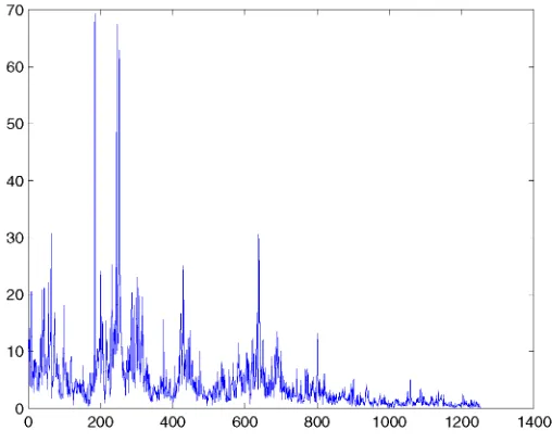
Hence we compare how correcting for microstructure noise im-proves the forecasts of future corrected increments and con-siderHequal to 1 week. Note that we consider uncorrected and corrected measures of quadratic variation on both sides of (1). The specifications of the polynomials were further discussed by Ghysels, Sinko, and Valkanov (2003). They discussed sev-eral alternative parametric specifications for the polynomials; we use their so-called “beta polynomial,” which are particularly suitable for the application at hand. The MSFT stock is used as an empirical example. Figure 1 displays the daily volatility dy-namics using theRV(AC5 min)
1 volatility measure for the sample considered by Hansen and Lunde. The time series plot clearly
Figure 1. Daily RVAC(5 min)
1 Realized Volatility. The figure shows daily
RV with an AC1noise-correction scheme. The 753rd observation is the
2002 end-of-year observation. The mean of the first 3 years is 6.18; the mean of the second 2 years is 1.74.
demonstrates that volatility dynamics of the first part of the sample are quite different from those of the second one. There is evidence of a structural change or regime switch, which leads us to study not only the entire sample, but also two subsam-ples, 3 years and 2 years long. The sample mean of the daily series for the first 3 years (the first 753 observations) is 6.15, whereas that for the last 2 years (the last 501 observations) is 1.47.
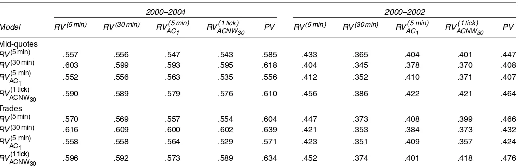
Our analysis covers two sample sizes and two measures of stock returns. We start with the entire sample (January 3, 2000– December 31, 2004). Next, we consider the subsample from January 3, 2000 to December 31, 2002. The returns are com-puted using mid-quote prices and trading prices. The results, covering both definitions of returns and covering both samples, are given in Table 1, where each row corresponds to the same left-side variable discussed earlier but with different explana-tory variables and sample sizes.
In this section we discuss the explanatory power of the dif-ferentRVxymeasures of the quadratic variation, that is, first four columns for each sample in the table. The main finding is that there is no significant difference between unadjusted and ad-justed predictors. Moreover, the unadad-justedRV(5 min) measure has the best explanatory power across all models and samples except for the whole sample, where the model with RV(AC5 min)
1 does marginally better (with a difference of only 1.1%). The results are robust for different data samples and different re-turn measures. Hence, from MSFT, we find that noise-corrected volatility measures performs on average worse than unadjusted 5 minutes volatility measure. One explanation is that the signal-to-noise ratio is high, and, in terms of the MSE, the uncorrected measure is better than the corrected ones. Another explanation is that the MIDAS regression is extremely effective in extract-ing the signal from the daily realized volatility measures, and noise correction only reduces the explanatory power of the re-gression.
194 Journal of Business & Economic Statistics, April 2006
Table 1. R2Comparison of MIDAS Models for 1-Week Horizon, MSFT Stock 2000–2004 2000–2002
NOTE: Each entry in the table corresponds to theR2for different models (1) and (2) and different estimation samples. The whole sample covers January 3, 2000–December 31, 2004. Subsample
2000–2002 covers January 3, 2000–December 31, 2002. The regressions are run on a weekly (5 days) data sampling scheme. The names of the variables are consistent with the notation in Hansen and Lunde’s article. Every column corresponds to the explanatory power of the different left-side variables for the same right-side variable.
3. WHY QUADRATIC VARIATION?
RV is not the only measure of volatility. Ghysels et al. (2006) found that volatility can be forecasted using daily regressors other than squared returns. They showed that better in-sample and out-of-sample estimates of the volatility are obtained when the predictors on the right side are daily absolute returns, daily RVs, daily ranges, and daily realized powers. We provide the exact definitions of these predictors here. The daily realized volatility, daily ranges, and daily realized powers are obtained from intradaily (5-minute) data of the Dow Jones index re-turns over April 1993–October 2003. Ghysels et al. (2006) showed that the best overall predictor of conditional volatil-ity is the realized power and that, not surprisingly, better fore-casts are obtained at shorter (weekly) horizons. This empirical evidence was corroborated by theoretical and further empiri-cal work by Forsberg and Ghysels (2004), who used the the-oretical framework of Barndorff-Nielsen and Shephard (2001) involving a non-Gaussian Ornstein–Uhlenbeck (OU) volatility process with nonnegative Lévy increments. Within this diffu-sion framework, Forsberg and Ghysels showed that realized power is expected to be the best predictor. To appraise how microstructure-corrected QV compares with the measures con-sidered by Ghysels et al. (2006), we examine
RVxy(t+H,t)
where PV$(m) is the power variation or the sum of intradaily absolute returns.
We use the same data as in the previous section. PV is ob-tained using daily aggregation of 5-minutes returns. The results for the PV appear in the 5th and 10th columns of the Table 1. Consistent with Ghysels et al. (2006) and Forsberg and Ghysels (2004), PV appears not only to be the best predictor compared with uncorrected predictors, but also to have the best explana-tory power for all models except one. The R2’s for PV are
most often between 1–4% higher for 1-week-ahead predictions. These results become even more dramatic at long horizons (not reported here). Hence, combining this with the results from the previous section, we can conclude that, on average, noise cor-rection does not appear to be important for volatility predic-tion.
Correcting PV for microstructure noise is a much harder problem than correcting QV. By analogy with QV, the correc-tion may perhaps not improve much on the performance of fore-casting.
To be fair, we have changed the objective function. Hansen and Lunde try to find the best filter that eliminates microstruc-ture noise, whereas our objective function is to predict fumicrostruc-ture volatility. Arguably, predicting future volatility is one of the ul-timate objectives. Our findings reported here can be robustified; we have computed results for stocks other than MSFT, and they yield very much the same type of results as those reported in Ta-ble 1. Nevertheless, more work is needed to get the full picture; we are doing this (Ghysels and Sinko 2005).
ACKNOWLEDGMENTS
The authors thank Peter Hansen and Asger Lunde for provid-ing the data used in this comment.
ADDITIONAL REFERENCES
Forsberg, L., and Ghysels, E. (2004), “Why Do Absolute Returns Predict Volatility so Well?” working paper, University of North Carolina, Dept. of Economics.
Ghysels, E. (1988), “A Study Towards a Dynamic Theory of Seasonality for Economic Time Series,”Journal of the American Statistical Association, 85, 168–172.
(1996), “On the Economics and Econometrics of Seasonality,” in Ad-vances in Econometrics, Sixth World Congress, ed. C. A. Sims, Cambridge, U.K.: Cambridge University Press, pp. 257–316.
Ghysels, E., and Osborn, E. (2001),The Econometric Analysis of Seasonal Time Series, Cambridge, U.K.: Cambridge University Press.
Ghysels, E., and Sinko, A. (2005), “Volatility Prediction and Microstructure Noise,” working paper, University of North Carolina, Dept. of Economics. Ghysels, E., Sinko, A., and Valkanov, R. (2003), “MIDAS Regressions: Further
Results and New Directions,”Econometric Reviews, forthcoming.