Micro, Nanosystems and Systems on Chips

(1)

(2)

(3)

Micro, Nanosystems

and Systems on Chips

Modeling, Control and Estimation

(4)

First published 2010 in Great Britain and the United States by ISTE Ltd and John Wiley & Sons, Inc. Apart from any fair dealing for the purposes of research or private study, or criticism or review, as permitted under the Copyright, Designs and Patents Act 1988, this publication may only be reproduced, stored or transmitted, in any form or by any means, with the prior permission in writing of the publishers, or in the case of reprographic reproduction in accordance with the terms and licenses issued by the CLA. Enquiries concerning reproduction outside these terms should be sent to the publishers at the undermentioned address:

ISTE Ltd John Wiley & Sons, Inc. 27-37 St George’s Road 111 River Street

London SW19 4EU Hoboken, NJ 07030

UK USA

www.iste.co.uk www.wiley.com

The rights of Alina Voda to be identified as the author of this work have been asserted by her in accordance with the Copyright, Designs and Patents Act 1988.

Library of Congress Cataloging-in-Publication Data

Micro, nanosystems, and systems on chips : modeling, control, and estimation / edited by Alina Voda. p. cm.

Includes bibliographical references and index. ISBN 978-1-84821-190-2

1. Microelectromechanical systems. 2. Systems on a chip. I. Voda, Alina. TK7875.M532487 2010

621.381--dc22

2009041386 British Library Cataloguing-in-Publication Data

A CIP record for this book is available from the British Library ISBN 978-1-84821-190-2

(5)

Introduction . . . xi

PARTI. MINI ANDMICROSYSTEMS . . . 1

Chapter 1. Modeling and Control of Stick-slip Micropositioning Devices . 3 Micky RAKOTONDRABE, Yassine HADDAB, Philippe LUTZ 1.1. Introduction . . . 3

1.2. General description of stick-slip micropositioning devices . . . 4

1.2.1. Principle . . . 4

1.2.2. Experimental device . . . 5

1.3. Model of the sub-step mode . . . 6

1.3.1. Assumptions . . . 6

1.3.2. Microactuator equation . . . 8

1.3.3. The elastoplastic friction model . . . 8

1.3.4. The state equation . . . 10

1.3.5. The output equation . . . 11

1.3.6. Experimental and simulation curves . . . 12

1.4. PI control of the sub-step mode . . . 13

1.5. Modeling the coarse mode . . . 15

1.5.1. The model . . . 16

1.5.2. Experimental results . . . 17

1.5.3. Remarks . . . 17

1.6. Voltage/frequency(U/f)proportional control of the coarse mode . . . 18

1.6.1. Principle scheme of the proposed controller . . . 20

1.6.2. Analysis . . . 20

1.6.3. Stability analysis . . . 24

1.6.4. Experiments . . . 25

1.7. Conclusion . . . 26

(6)

Chapter 2. Microbeam Dynamic Shaping by Closed-loop Electrostatic

Actuation using Modal Control . . . 31

Chady KHARRAT, Eric COLINET, Alina VODA 2.1. Introduction . . . 31

2.2. System description . . . 34

2.3. Modal analysis . . . 36

2.4. Mode-based control . . . 40

2.4.1. PID control . . . 42

2.4.2. FSF-LTR control . . . 43

2.6. Bibliography . . . 53

PARTII. NANOSYSTEMS ANDNANOWORLD . . . 57

Chapter 3. Observer-based Estimation of Weak Forces in a Nanosystem Measurement Device . . . 59

Gildas BESANÇON, Alina VODA, Guillaume JOURDAN 3.1. Introduction . . . 59

3.2. Observer approach in an AFM measurement set-up . . . 61

3.2.1. Considered AFM model and force measurement problem . . . 61

3.2.2. Proposed observer approach . . . 63

3.2.3. Experimental application and validation . . . 65

3.3. Extension to back action evasion . . . 71

3.3.1. Back action problem and illustration . . . 71

3.3.2. Observer-based approach . . . 73

3.3.3. Simulation results and comments . . . 76

3.5. Acknowledgements . . . 81

Chapter 4. Tunnel Current for a Robust, High-bandwidth and Ultra-precise Nanopositioning . . . 85

Sylvain BLANVILLAIN, Alina VODA, Gildas BESANÇON 4.1. Introduction . . . 85

4.2. System description . . . 87

4.2.1. Forces between the tip and the beam . . . 88

4.3. System modeling . . . 89

4.3.1. Cantilever model . . . 89

4.3.2. System actuators . . . 90

4.3.3. Tunnel current . . . 92

4.3.4. System model . . . 93

(7)

4.4. Problem statement . . . 97

4.4.1. Robustness and non-linearities . . . 97

4.4.2. Experimental noise . . . 98

4.5. Tools to deal with noise . . . 100

4.5.1. Kalman filter . . . 100

4.5.2. Minimum variance controller . . . 100

4.6. Closed-loop requirements . . . 102

4.6.1. Sensitivity functions . . . 102

4.6.2. Robustness margins . . . 102

4.6.3. Templates of the sensibility functions . . . 103

4.7. Control strategy . . . 105

4.7.1. Actuator linearization . . . 106

4.7.2. Sensor approximation . . . 106

4.7.3. Kalman filtering . . . 108

4.7.4. RST₁synthesis . . . 108

4.7.5.zreconstruction . . . 110

4.7.6. RST₂synthesis . . . 110

4.8. Results . . . 111

4.8.1. Position control . . . 111

4.8.2. Distancedcontrol . . . 113

4.8.3. Robustness . . . 114

Chapter 5. Controller Design and Analysis for High-performance STM . . 121

Irfan AHMAD, Alina VODA, Gildas BESANÇON 5.1. Introduction . . . 121

5.2. General description of STM . . . 123

5.2.1. STM operation modes . . . 123

5.2.2. Principle . . . 124

5.3. Control design model . . . 127

5.3.1. Linear approximation approach . . . 127

5.3.2. Open-loop analysis . . . 129

5.3.3. Control problem formulation and desired performance for STM . 131 5.4.H∞controller design . . . 131

5.4.1. General control problem formulation . . . 131

5.4.2. GeneralH∞algorithm . . . 133

5.4.3. Mixed-sensitivityH∞control . . . 134

5.4.4. Controller synthesis for the scanning tunneling microscope . . . . 135

5.4.5. Control loop performance analysis . . . 137

5.5. Analysis with system parametric uncertainties . . . 139

5.5.1. Uncertainty modeling . . . 140

(8)

5.6. Simulation results . . . 142

5.7. Conclusions . . . 143

Chapter 6. Modeling, Identi_ﬁcation and Control of a Micro-cantilever Array . . . 149

Scott COGAN, Hui HUI, Michel LENCZNER, Emmanuel PILLET, Nicolas RATTIER, Youssef YAKOUBI 6.1. Introduction . . . 150

6.2. Modeling and identification of a cantilever array . . . 151

6.2.1. Geometry of the problem . . . 151

6.2.2. Two-scale approximation . . . 151

6.2.3. Model description . . . 153

6.2.4. Structure of eigenmodes . . . 154

6.2.5. Model validation . . . 155

6.2.6. Model identification . . . 159

6.3. Semi-decentralized approximation of optimal control applied to a cantilever array . . . 164

6.3.1. General notation . . . 164

6.3.2. Reformulation of the two-scale model of cantilever arrays . . . . 164

6.3.3. Model reformulation . . . 166

6.3.4. Classical formulation of the LQR problem . . . 167

6.3.5. Semi-decentralized approximation . . . 168

6.3.6. Numerical validation . . . 173

6.4. Simulation of large-scale periodic circuits by a homogenization method 175 6.4.1. Linear static periodic circuits . . . 176

6.4.2. Circuit equations . . . 178

6.4.3. Direct two-scale transformTE . . . 179

6.4.4. Inverse two-scale transformT−₁ E . . . 180

6.4.5. Two-scale transformTN . . . 182

6.4.6. Behavior of ‘spread’ analog circuits . . . 182

6.4.7. Cell equations (micro problem) . . . 184

6.4.8. Reformulation of the micro problem . . . 187

6.4.9. Homogenized circuit equations (macro problem) . . . 188

6.4.10. Computation of actual voltages and currents . . . 189

6.6. Appendix . . . 193

Chapter 7. Fractional Order Modeling and Identi_ﬁcation for Electrochemical Nano-biochip . . . 197

Abdelbaki DJOUAMBI, Alina VODA, Pierre GRANGEAT, Pascal MAILLEY 7.1. Introduction . . . 197

(9)

7.2.1. Brief review of fractional differentiation . . . 199

7.2.2. Fractional order systems . . . 201

7.3. Prediction error algorithm for fractional order system identification . . 202

7.4. Fractional order modeling of electrochemical processes . . . 206

7.5. Identification of a real electrochemical biochip . . . 209

7.5.1. Experimental set-up . . . 209

7.5.2. Fractional order model identification of the considered biochip . . 213

PARTIII. FROMNANOWORLD TOMACRO ANDHUMANINTERFACES . 221 Chapter 8. Human-in-the-loop Telemicromanipulation System Assisted by Multisensory Feedback . . . 223

Mehdi AMMI, Antoine FERREIRA 8.1. Introduction . . . 224

8.2. Haptic-based multimodal telemicromanipulation system . . . 225

8.2.1. Global approach . . . 225

8.2.2. Telemicromanipulation platform and manipulation protocol . . . . 226

8.3. 3D visual perception using virtual reality . . . 228

8.3.1. Limitations of microscopy visual perception . . . 228

8.3.2. Coarse localization of microspheres . . . 229

8.3.3. Fine localization using image correlation techniques . . . 229

8.3.4. Subpixel localization . . . 230

8.3.5. Localization of dust and impurities . . . 233

8.3.6. Calibration of the microscope . . . 234

8.3.7. 3D reconstruction of the microworld . . . 234

8.4. Haptic rendering for intuitive and efficient interaction with the micro-environment . . . 237

8.4.1. Haptic-based bilateral teleoperation control . . . 237

8.4.2. Active operator guidance using potential fields . . . 239

8.4.3. Model-based local motion planning . . . 243

8.4.4. Force feedback stabilization by virtual coupling . . . 243

8.5. Evaluating manipulation tasks through multimodal feedback and assistance metaphors . . . 246

8.5.1. Approach phase . . . 246

Chapter 9. Six-dof Teleoperation Platform: Application to Flexible Molecular Docking . . . 257

(10)

9.2. Proposed approach . . . 261

9.2.1. Molecular modeling and simulation . . . 261

9.2.2. Flexible ligand and flexible protein . . . 262

9.2.3. Force feedback . . . 263

9.2.4. Summary . . . 265

9.3. Force-position control scheme . . . 266

9.3.1. Ideal control scheme without delays . . . 266

9.3.2. Environment . . . 268

9.3.3. Transparency . . . 269

9.3.4. Description of a docking task . . . 270

9.3.5. Influence of the effort scaling factor . . . 272

9.3.6. Influence of the displacement scaling . . . 274

9.3.7. Summary . . . 276

9.4. Control scheme for high dynamical and delayed systems . . . 277

9.4.1. Wave transformation . . . 277

9.4.2. Virtual damper using wave variables . . . 278

9.4.3. Wave variables without damping . . . 282

9.4.4. Summary . . . 286

9.5. From energy description of a force field to force feeling . . . 287

9.5.1. Introduction . . . 287

9.5.2. Energy modeling of the interaction . . . 287

9.5.3. The interaction wrench calculation . . . 291

9.5.4. Summary . . . 293

List of Authors . . . 301

(11)

Micro and nanosystems represent a major scientific and technological challenge, with actual and potential applications in almost all fields of human activity. From the first physics and philosophical concepts of atoms, developed by classical Greek and Roman thinkers such as Democritus, Epicurus and Lucretins some centuries BC at the dawn of the scientific era, to the famous Nobel Prize Feynman conference 50 years ago (“There is plenty of room at the bottom”), phenomena at atomic scale have incessantly attracted the human spirit. However, to produce, touch, manipulate and create such atomistic-based systems has only been possible during the last 50 years as the appropriate technologies became available.

Books on micro- and nanosystems have already been written and continue to appear. They focus on the physics, chemical, technological and biological concepts, problems and applications. The dynamical modeling, estimation and feedback control are not classically addressed in the literature on miniaturization. However, these are innovative and efficient approaches to explore and improve; new small-scale systems could even be created.

The instruments for measuring and manipulating individual systems at molecular and atomic scale cannot be imagined without incorporating very precise estimation and feedback control concepts. On the other hand, to make such a dream feasible, control system methods have to adapt to unusual systems governed by different physics than the macroscopic systems. Phenomena which are usually neglected, such as thermal noise, become an important source of disturbances for nanosystems. Dust particles can represent obstacles when dealing with molecular positioning. The influence of the measuring process on the measured variable, referred to as back action, cannot be ignored if the measured signal is of the same order of magnitude as the measuring device noise.

(12)

this scale. The aim of this book is to present how concepts from dynamical control systems (modeling, estimation, observation, identification and feedback control) can be adapted and applied to the development of original very small-scale systems and to their human interfaces.

All the contributions have a model-based approach in common. The model is a set of dynamical system equations which, depending on its intended purpose, is either based on physics principles or is a black-box identified model or an energy (or potential field) based model. The model is then used for the design of the feedback control law, for estimation purposes (parameter identification or observer design) or for human interface design.

The applications presented in this book range from micro- and nanorobotics and biochips to near-field microscopy (Atomic Force and Scanning Tunneling Micro-scopes), nanosystems arrays, biochip cells and also human interfaces.

The book has three parts. The first part is dedicated to mini- and microsystems, with two applications of feedback control in micropositioning devices and microbeam dynamic shaping.

The second part is dedicated to nanoscale systems or phenomena. The fundamental instrument which we are concerned with is the microscope, which is either used to analyze or explore surfaces or to measure forces at an atomic scale. The core of the microscope is a cantilever with a sharp tip, in close proximity to the sample under analysis. Several chapters of the book treat different aspects related to the microscopy: force measurement at nanoscale is recast as an observer design, fast and precise nano-positioning is reached by feedback control design and cantilever arrays can be modeled and controlled using a non-standard approach. Another domain of interest is the field of biochips. A chapter is dedicated to the identification of a non-integer order model applied to such an electrochemical transduction/detection cell.

The third part of the book treats aspects of the interactions between the human and nanoworlds through haptic interfaces, telemanipulation and virtual reality.

(13)

(14)

Modeling and Control of Stick-slip

Micropositioning Devices

The principle of stick-slip motion is highly appreciated in the design of micro-positioning devices. Indeed, this principle offers both a very high resolution and a high range of displacement for the devices. In fact, stick-slip motion is a step-by-step motion and two modes can therefore be used: the step-by-stepping mode (for coarse positioning) and the sub-step mode (for fine positioning). In this chapter, we present the modeling and control of micropositioning devices based on stick-slip motion principle. For each mode (sub-step and stepping), we describe the model and propose a control law in order to improve the performance of the devices. Experimental results validate and confirm the results in the theoretical section.

1.1. Introduction

In microassembly and micromanipulation tasks, i.e. assembly or manipulation of objects with submillimetric sizes, the manipulators should achieve a micrometric or submicrometric accuracy. To reach such a performance, the design of microrobots and micromanipulators is radically different from the design of classical robots. Instead of using hinges that may introduce imprecision, active materials are preferred. Piezoelectric materials are highly prized because of the high resolution and the short response time they can offer.

In addition to the high accuracy, a large range of motion is also important in microassembly/micromanipulation tasks. Indeed, the pick-and-place of small objects

(15)

may require the transportation of the latter over a long distance. To execute tasks with high accuracy and over a high range of displacement, micropositioning devices and microrobots use embedded (micro)actuators. According to the type of microactuators used, there are different motion principles that can be used e.g. the stick-slip motion principle, the impact drive motion principle and the inch-worm motion principle. Each of these principles provides a step-by-step motion. The micropositioning device analyzed and experimented upon in this chapter is based on the stick-slip motion principle and uses piezoelectric microactuators.

Stick-slip micropositioning devices can work with two modes of motion: the coarse mode which is for long-distance positioning and the sub-step mode which is for fine positioning. This chapter presents the modeling and the control of the micropositioning device for both fine and coarse modes.

First we describe the micropositioning device. The modeling and control in fine mode are then analyzed. We then present the modeling in coarse mode, and end the chapter by describing control of the device in coarse mode.

1.2. General description of stick-slip micropositioning devices

1.2.1. Principle

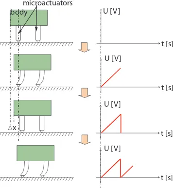
Figure 1.1a explains the functioning of the stick-slip motion principle. In the figure, two microactuators are embedded onto a body to be moved. The two microactuators are made of a smart material. Here, we consider piezoelectric microac-tuators.

If we apply a ramp voltage to the microactuators, they slowly bend. As the bending acceleration is low, there is an adherence between the tips of the microactuators and the base (Figure 1.1b). If we reset the voltage, the bending of the legs is also abruptly halted. Because of the high acceleration, sliding occurs between their tips and the base. A displacement∆xof the body is therefore obtained (Figure 1.1c). Repeating the sequence using a sawtooth voltage signal makes the body perform a step-by-step motion. The corresponding motion principle is called stick-slip. The amplitude of a step is defined by the sawtooth voltage amplitude and the speed of the body is defined by both the amplitude and the frequency. The step value indicates the positioning resolution.

(16)

Δx body

microactuators

t [s] U [V]

Figure 1.1.Stick-slip principle: (a–c) stepping mode and (d) scanning mode

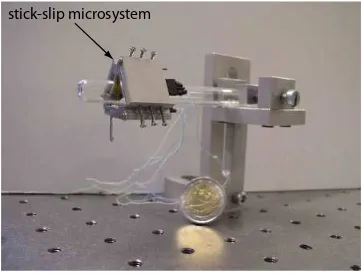
1.2.2. Experimental device

The positioning device experimented upon in this paper, referred to as triangular RING (TRING) module, is depicted in Figure 1.2. It can perform a linear and an angular motion on the base (a glass tube) independently. Without loss of generality, our experiments are carried out only in linear motion. To move the TRING-module, six piezoelectric microactuators are embedded. Details of the design and development of the TRING-module are given in [RAK 06, RAK 09] while the piezoelectric microactuators are described in [BER 03].

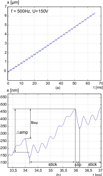
To evaluate the step of the device, we apply a sawtooth signal to its microactuators. The measurements were carried out with an interferometer of 1.24nm resolution. Figure 1.3a depicts the resulting displacement at amplitude 150V and frequency 500Hz. We note that the step is quasi-constant during the displacement. Figure 1.3b is a zoomed image of one step. The oscillations during the stick phase are caused by the dynamics of the microactuators and the mass of the TRING-module. The maximal step, obtained with150V, is about200nm. Decreasing the amplitude will decrease the value of the step and increase the resolution of the micropositioning device. As an example, with U = 75V the step is approximatively 70nm. However, the step efficiency is constant whatever the value of the amplitude. It is defined as the ratio of the gained step to the amplitude of the sawtooth voltage [DRI 03]:

ηstep= step

(17)

stick-slip microsystem

Figure 1.2.A photograph of the TRING-module

As introduced above, two modes of displacement are possible: the fine and the coarse modes. In the next sections, the fine mode of the TRING-module is first modeled and controlled. After that, we will detail the modeling and the control in coarse mode, all with linear motion.

1.3. Model of the sub-step mode

The sub-step modeling of a stick-slip micropositioning device is highly dependent upon the structure of microactuators. This in turn depends upon the required number of degrees of freedom and their kinematics, the structure of the device where they will be integrated and the structure of the base. For example, [FAT 95] and [BER 04] use two kinds of stick-slip microactuators to move the MICRON micropositioning device (5-dof) and the MINIMAN micropositioning device (3-(5-dof). Despite this dependence of the model on the microactuator’s structure, as long as the piezoelectric microactuator is operating linearly, the sub-step model is still linear [RAK 09].

During the modeling of the sub-step mode, it is of interest to include the state of the friction between the microactuators and the base. For example, it is possible to control it to be lower than a certain value to ensure the stick mode. There are several models of friction according to the application [ARM 94], but the elastoplastic model [DUP 02] is best adapted to the sub-step modeling. The model of the sub-step mode is therefore linear and has an order at least equal to the order of the microactuator model.

1.3.1. Assumptions

(18)

0 10 20 30 40 50 60 70 0

1 2 3 4 5 6

(a)

(b) 7

f = 500Hz, U=150V x [µm]

x [nm] t [ms]

t [ms] 33,5 34 34,5 35 35,5 36 36,5 37 3100

3150 3200 3250 3300 3350 3400 3450 3500 3550

step

Δamp

stick slip stick

Figure 1.3.Linear displacement measurement of the TRING-module using an interferometer: (a) a series of stick-slip motion obtained withU = 150_{V and}_f= 500_{Hz and (b) vibrations}

inside a step obtained withU= 150_{V and}_f= 60_Hz

preload charge is the vertical force that maintains the device on the base. The base is considered to be rigid and we assume that no vibration affects it because we work in the stick mode. Indeed, during this mode, the tip of the microactuator and the base are fixed and shocks do not cause vibration.

(19)

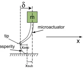
1.3.2. Microactuator equation

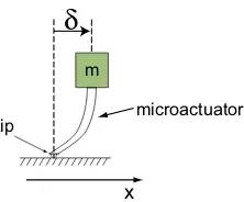
The different microactuators and the positioning device can be lumped into one microactuator supporting a body (Figure 1.4).

m

microactuator tip

x

δ

Figure 1.4.Schematic of the microactuator

If the microactuator works in a linear domain, a second-order lumped model is:

a2δ¨+a1δ˙+δ=dpU+spFpiezo (1.2)

where δis the deflection of the microactuator,ai are the parameters of the dynamic parts, dp is the piezoelectric coefficient, sp is the elastic coefficient and Fpiezo is the external force applied to the microactuator. It may be derived from external disturbance (manipulation force, etc.) or internal stresses between the base and the microactuator.

1.3.3. The elastoplastic friction model

The elastoplastic friction model was proposed by Dupont et al. [DUP 02] and is well adapted for stick-slip micropositioning devices. Consider a block that moves along a base (Figure 1.5a). If the forceF applied to the block is lower than a certain value, the block does not move. This corresponds to a stick phase. If we increase the force, the block starts sliding and the slip phase is obtained.

In the elastoplastic model, the contact between the block and the base are lumped in a medium asperity model (Figure 1.5b). LetGbe the center of gravity of the block andxits motion. During the stick phase, the medium asperity bends. As there is no sliding (w˙ = 0), the motion of the block corresponds only to the deflectionxaspof the asperity:x=xasp. This motion is elastic; when the force is removed, the deflection becomes null.

(20)

x

Figure 1.5.(a) A block that moves along a base and (b) the contact between the block and the base can be approximated by a medium asperity

w. Whilew˙ = 0, the deflectionxaspcontinues to vary. This phase is elastic because ofxaspbut also plastic because ofw.

IfFis increased further,xasptends to a saturation calledxssasp(steady state) and the speedx˙ of the block is equal tow˙ = 0. This phase is called plastic because removing the force will not reset the block to its initial position.

The equations describing the elastoplastic model are:

x = xaps+w

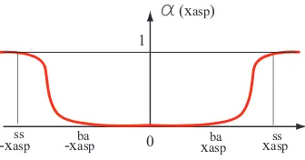
whereN designates the normal force applied to the block,ρ0andρ2are the Coulomb and the viscous parameters of the friction, respectively, ρ1 provides damping for tangential compliance andα(xasp,x˙)is a function which determines the phase (stick or slip). Figure 1.6 provides an example of allure ofα.

α

_(xasp)

(21)

For stick-slip devices working in the sub-step mode, there is no sliding and so ˙

w= 0. In addition, the coefficientsρ1andρ2are negligible because the friction is dry (there is no lubricant). Assuming that the initial value isw= 0, the friction equations of stick-slip devices in the stick mode are:

ff = −N ρ0xasp

x = xasp

˙

x = x˙asp. (1.4)

1.3.4. The state equation

To compute the model of the stick-slip micropositioning device in a stick mode, the deformation of the microactuator (equation (1.2)) and the friction model (equation (1.4)) are used. Figure 1.7 represents the same image as Figure 1.4 with the contact between the tip of the microactuator and the base enlarged. According to the figure, the displacementxsubcan be determined by combining the microactuator equationδand the friction statexaspusing dynamic laws [RAK 09].

m

Figure 1.7.An example of allure ofα

The state equation of the TRING-module is therefore:

d

(22)

– the states of the electromechanical part: the deflection δ of the piezoelectric microactuator and the corresponding derivative_δ˙_{; and}

– the states of the friction part: the deflection of a medium asperityxasp and the corresponding derivativex˙asp.

The following values have been identified and validated for the considered system [RAK 09]:

The output equation is defined as

where T is the friction andxsub is the displacement of the massmduring the stick mode. xsub corresponds to the fine position of the TRING device. The different parameters are defined:

C11 = −1,596

C12 = −0.32

C13 = −1,580,462,303

(23)

1.3.6. Experimental and simulation curves

In the considered application, we are interested in the control of the position. We therefore only consider the outputxsub. From the previous state and output equations, we derive the transfer function relating the applied voltage andxsub:

GxsubU =

wheresis the Laplace variable.

To compare the computed modelGxsubU and the real system, a harmonic analysis is performed by applying a sine input voltage to the TRING-module. The chosen amplitude of the sine voltage is75V instead of150V. Indeed, with a high amplitude the minimum frequency from which the drift (and then the sliding mode) starts is low. In the example of Figure 1.8, a frequency of2250Hz leads to a drift when the amplitude is150V while a frequency of5000Hz does not when amplitude is75V. The higher the amplitude, the higher the acceleration is and the higher the risk of sliding (drift). When the TRING-module slides, the sub-step model is no longer valuable.

0.0165 0.017 0.0175 0.018 0.0185 0.019 −20

sine voltage U=75V f=5000Hz

t [s] _(b) _{t [s]}

100 sine voltage U=150V f=2250Hz

Figure 1.8.Harmonic experiment: (a) outbreak of a drift of the TRING positioning system (sliding mode) and (b) stick mode

(24)

102 103 104 105 106 −250

−240 −230 −220 −210 −200 −190 −180 −170 −160

pulsation [rad/s] magnitude [dB]

simulation experimental

curve

Figure 1.9.Comparison of the simulation of the developed model and the experimental results

1.4. PI control of the sub-step mode

The aim of the sub-step control is to improve the performance of the TRING-module during a highly accurate task and to eliminate disturbances (e.g. manipulation force, adhesion forces and environmental disturbances such as temperature). Indeed, when positioning a microcomponent such as fixing a microlens at the tip of an optical fiber [GAR 00], the manipulation force can disturb the positioning task and modify its accuracy. In addition, the numerical values of the model parameters may contain uncertainty. We therefore present here the closed-loop control of the fine mode to introduce high stability margins.

The sub-step functioning requires that the derivativedU/dtof the voltage should be inferior to a maximum slope_U˙_{max. To ensure this, we introduce a rate limiter in} the controller scheme as depicted in Figure 1.10.

Usat

U xsub

xsub reference

stick-slip device +

-controller rate limiter

Figure 1.10.Structure of the closed-loop system

(25)

First, we trace the Black–Nichols diagram of the open-loop systemGxsubU, as

Frequency (rad/sec): 5.76e+003

Figure 1.11.Black–Nichols diagram ofGxsubU

Let

be the transfer function of the controller, where Kp and Ki = 1/Ti are the proportional and the integrator gains, respectively. The 60◦ of phase margin is obtained if the new open-loop transfer function KPI ×GxU has a Black–Nichols diagram which cuts the 0dB horizontal axis at 240◦. This can be obtained by computing a corrector KPI that adjusts the data depicted in Figure 1.11 to that required. Using the computation method presented in [BOU 06], we find:

Kp = 383,749,529

Ki = 7,940. (1.11)

The controller has been implemented following that depicted in Figure 1.10. The reference displacement is a step input signalxref

(26)

t [s] x [nm]

(a)

(b) Phase [°]

Gain [dB]

0 10 20 30 40 50 60 70 80 −20

0 20 40 60 80 100 120

step response (with a rate limiter)

180 225 270

−100 −50 0 50 100 150 200

0 dB 6 dB 3 dB

1 dB 0.5 dB 0.25 dB 60°

Figure 1.12.Results of the PI control of the TRING-module in sub-step functioning

Figure 1.12b shows the Black–Nichols diagram of the closed-loop system and indicates the margin phase. According to the figure, the margin gain is50dB. These robustness margins are sufficient to ensure the stability of the closed-loop system regarding the uncertainty of the parameters and of the structure of the developed model. Finally, the closed-loop control ensures these performances when external disturbances occur during the micromanipulation/microassembly tasks. A disturbance may be of an environmental type (e.g. temperature variation) or a manipulation type (e.g. manipulation force).

1.5. Modeling the coarse mode

(27)

discusses the modeling and control of the coarse mode. The presented results are applicable to stepping systems.

1.5.1. The model

First, let us study one step. For that, we first apply a ramp input voltage up toU. If the slope of the ramp is weak, there is no sliding between the tip of the microactuators and the base. Using the model in the stick mode, the displacement of the device is defined:

xsub(s) =GxsubU(s)×U(s). (1.12)

To obtain a step, the voltage is quickly reduced to zero. The resulting stepxstepis smaller than the amplitudexsubthat corresponds to the last value ofU (Figure 1.13a). We denote this amplitudexU

sub. We then have:

xstep=xUsub−∆back. (1.13)

t [s]

T T 2T 3T

x [µm]

(a) (b)

Δ

back

x x

x_sub sub

U

step

t [s] x [mm]

v [mm/s]

Figure 1.13.(a) Motion of a stick-slip system and (b) speed approximation

If we assume that backlash∆backis dynamically linear relative to the amplitude U, the step can be written as:

xstep(s) =Gstep(s)×U(s) (1.14)

where Gstep is a linear transfer function. When the sequence is repeated with a frequencyf = 1/T, i.e. a sawtooth signal, the micropositioning device works in the stepping mode (coarse mode). During this mode, each transient part inside a step is no longer important. Instead, we are interested in the speed performance of the device over a large distance. To compute the speed, we consider the final value of a step:

xstep=α×U (1.15)

(28)

From Figure 1.13b and equation (1.15), we easily deduce the speed:

v=xstep

T =xstep×f. (1.16)

The speed is therefore bilinear in relation to the amplitudeU and the frequencyf of the sawtooth input voltage:

v=αf U. (1.17)

However, the experiments show that there is a deadzone in the amplitude inside which the speed is null. Indeed, if the amplitudeU is below a certain valueU0, the micropositioning system does not move in the stepping mode but only moves back and forth in the stick mode. To take into account this threshold, equation (1.15) is slightly modified and the final model becomes:

v= 0 if |U| ≤U0

v=αf(U−sgn(U)U0) if |U|> U0. (1.18)

1.5.2. Experimental results

The identification on the TRING-module givesα = 15.65×10−7mm V−1 and U0= 35V. Figure 1.14 summarizes the speed performances of the micropositioning system: simulation of the model using equation (1.18) and experimental result. During the experiments, the amplitudeU is limited to±150V in order to avoid the destruction of the piezoelectric microactutors. Figure 1.14a depicts the speed versus amplitude for three different frequencies. It shows that the experimental results fit the model simulation well. Figure 1.14b depicts the speed versus frequency. In this, the experimental results and the simulation curve correspond up to f ≈ 10kHz; above this frequency there are saturations and fluctuations.

1.5.3. Remarks

To obtain equation (1.14), we made the assumption that the backlash∆backwas linear relative to the amplitudeU, such that in the static mode we have∆back = KbackUwhereKbackis the static gain of the backlash. In fact, the backlash is pseudo-linear relative toU becauseKbackis dependent uponU.

LetxU

sub=GxsubU(0)Ube the static value ofxsubin the sub-step mode obtained using equation (1.12) and corresponding to an inputU, whereGxsubU(0)is a static gain. Substituting it into equation (1.13) and using equation (1.16), we have:

(29)

0 2 4 6 8 10 12 14 16

Figure 1.14.Speed performances of the micropositioning system (experimental results in solid lines and simulation of equation (1.18) in dashed lines): (a) speed versus the amplitudeUand

(b) speed versus the frequencyf

Comparing equation (1.19) and the second equation of equation (1.18), we demonstrate the pseudo-linearity of the backlash in relation toU:

Kback=GxsubU(0)−α

1.6. Voltage/frequency(U/f)proportional control of the coarse mode

(30)

A stick-slip device is a type of stepping motor, and so stepping motor control techniques may be used. The easiest control of stepping motors is the open-loop counter technique. This consists of applying the number of steps necessary to reach a final position. In this, no sensor is necessary but the step value should be exactly known. In stick-slip micropositioning devices, such a technique is not very convenient. In fact, the friction varies along a displacement and the step is not very predictible. Closed-loop controllers are therefore preferred.

In closed-loop techniques, a natural control principle is the following basic algorithm:

WHILE|xc−x| ≥stepDO apply 1 step

ENDWHILE (1.21)

where xc andxare the reference and the present positions of the stick-slip devices, respectively, and step is the value of one step. The resolution of the closed-loop system is equal to 1 step. If the accuracy of the sensor is lower than 1 step, a slight modification can be made:

WHILE|xc−x| ≥n×stepDO applyn×step

ENDWHILE. (1.22)

It is clear that for very precise positioning, the basic algorithm must be combined with a sub-step controller (such as the PI controller presented in the previous section). In that case, equation (1.21) is first activated during the coarse mode. When the error positionxc−xis lower than the value of a step, the controller is switched into the sub-step mode.

(31)

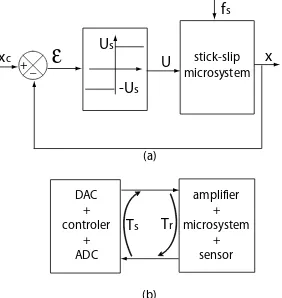
A technique based on the theory of dynamic hybrid systems has been used in [SED 03]. The mixture of the fine mode and the coarse mode actually constitutes a dynamic hybrid system. In the proposed technique, the hybrid system is first approximated by a continuous model by inserting a cascade with a hybrid controller. The approximation is called dehybridization. A PI-controller is then applied to the obtained continuous system.

In the following section, we propose a new controller scheme. In contrast to the dehybridization-based controller, the proposed scheme is very easy to implement because it does not require a hybrid controller. The proposed scheme always ensures the stability. The resolution that it provides is better than that of the basic algorithm. It will be shown that the controller is a globalization of three existing controllers: the bang-bang controller, the proportional controller and the frequency-proportional controller cited above.

1.6.1. Principle scheme of the proposed controller

The principle scheme of the controller is depicted in Figure 1.15. Basically, the principle is that the input signals (the amplitude and the frequency) are proportional to the error. This is why the proposed scheme is referred to as voltage/frequency (orU/f) proportional control. In Figure 1.15, the amplitude saturation limits any over-voltages that may destroy the piezoelectric microactuators. The frequency saturation limits the micropositioning system work inside the linear frequential zone. The controller parameters are the proportional gainsKU >0andKf >0.

stick-slip microsystem U

f

x xc

+ _

KU

absolute-value function

(saturationfunction) (saturation function)

Kf

| . |

ε

Figure 1.15.Principle scheme of theU/fproportional control

1.6.2. Analysis

Because of the presence of saturation in the controller scheme (Figure 1.15), different situations can occur [RAK 08] dependent upon the frequency and/or the amplitude being in the saturation zones. In this section, we analyze these situations.

(32)

1.6.2.1. Case a

In the first case, we assume that both the amplitude and the frequency are saturated, i.e.

KU|xc−x|> UsandKf|xc−x|> fs. (1.23)

This can be intepreted in two ways: the present position of the device is different from the reference position or the chosen proportional gains are very high. The equation of the closed-loop system in this case is obtained using the principle scheme in Figure 1.15 and equation (1.18). We have:

˙

x=αfs(Us−U0) sgn (xc−x). (1.24)

In such a case, the amplitudeUis switched betweenUsand−Usaccording to the sign of the error (Figure 1.16a). This case is therefore equivalent to a sign or bang-bang controller. With a sign control, there are oscillations. The frequency and the amplitude of these oscillations depend on the response timeTrof the process, on the refreshing timeTsof the controller and on the frequency saturationfs(Figure 1.16b). To minimize the oscillations, the use of realtime feedback systems is recommended.

(a)

(b) DAC

+ controler

+ ADC

amplifier + microsystem

+ sensor U

fs

Us

-Us

x xc

+ _

ε

Tr

Ts

Figure 1.16.Sign controller equivalence of theU/fcontroller

1.6.2.2. Case b

If the amplitudeUis lower than the thresholdU0regardless of frequency, i.e. if

U0> KU|xc−x|,∀f =Kf|xc−x|, (1.25)

(33)

1.6.2.3. Case c

In this case, the frequency is saturated while the amplitude is not. The condition corresponding to this case is:

Us≥KU|xc−x| andKf|xc−x|> fs. (1.26)

In such a case, the system is controlled by a classical proportional controller with gainKU (Figure 1.17).

U

fs

x xc

+ _

ε

KU

Figure 1.17.Voltage proportional control

The equation of the closed loop is easily obtained:

˙

x=αfs(KU(xc−x)−sgn (xc−x)U0). (1.27)

If we consider a positive reference positionxc >0and an initial valuex(t= 0) equal to zero, we obtain the Laplace transformation:

X= 1

1 + 1 αfsKUs

Xc− 1 KU 1 + 1

αfsKUs

U0. (1.28)

According to equation (1.28), the closed-loop process is a first-order dynamic system with a static gain equal to unity and a disturbance U0. The static error due to the disturbanceU0 is minimized when increasing the gainKU. Because the order is equal to that of the closed-loop system, this case is always stable.

1.6.2.4. Case d

Here we consider that the amplitude is saturated while the frequency is not, i.e.

KU|xc−x|> Usandfs≥Kf|xc−x|. (1.29)

(34)

f Us

x xc

+ _

ε

| . | Kf

Figure 1.18.Frequency proportional control

difference between this case and the controller proposed in [BRE 98] is that, in the latter, the controller is digital and based on an 8-bit counter.

Using Figure 1.18 and model (1.18), we have the non-linear differential model:

˙

x=αKf|xc−x|(Us−U0) sgn (xc−x) (1.30)

wherexcis the input andxis the output. Forxc>0and an initial valuex(t= 0) = 0, we deduce the transfer function from equation (1.30):

X Xc =

1 1 + _αK 1

f(Us−U0)s

. (1.31)

According to equation (1.31), the closed-loop process is a first-order system. Because the static gain is unity, there is no error static.

1.6.2.5. Case e

In this case, we consider that both the amplitude and the frequency are not saturated:

Us≥KU|xc−x| andfs≥Kf|xc−x|. (1.32)

Using Figure 1.15 and equation (1.18), we have:

˙

x=αKf|xc−x|(KU(xc−x)−sgn (xc−x)U0). (1.33)

The previous expression is equivalent to:

dx

dt = (αKf(U0−α)KfKU|xc−x|)x

(35)

Hence, the closed-loop system is equivalent to a first-order pseudo-linear system. Indeed, equation (1.34) has the form:

dx

dt =A(xc, x)x+B(xc, x)xc. (1.35)

1.6.3. Stability analysis

Here we analyze the stability of the closed-loop system. We note that all the cases stated above may appear during a displacement according to the values ofKU,Kf and the error(xc−x). To analyze the stability, we assumexc = 0andx(t= 0)>0 without loss of generality. In addition, let us divide the whole displacement into two phases as depicted in Figure 1.19:

– Phase 1: concerns the amplitude and the frequency in saturation. This corresponds to the error (xc−x) being initially high (case a). The speed is then constant.

– Phase 2: the error becomes smaller and the speed is not yet constant (equivalent to the rest of the cases).

Figure 1.19.Division of the displacement into two phases

According to equation (1.18), the device works in a quasi-static manner. Hence, there is no acceleration and any one case does not influence the succeeding case. Conditions relative to initial speed are not necessary so we can analyze phase 2 independently of phase 1. In phase 2, there are two sub-phases:

– Phase 2.1: either the frequency is in saturation but not the amplitude (case c) or the amplitude is in saturation but not the frequency (case d).

– Phase 2.2: neither the frequency nor the amplitude are in saturation (case e).

(36)

xc= 0andx(t= 0)>0, we have:

dx

dt =−αKfx(KUx−U0). (1.36)

To prove the stability, we use the direct method of Lyapunov. A systemdx/dt= f(x, t)is stable if there exists a Lyapunov functionV(x)that satisfies:

V(x= 0) = 0

V(x)>0 ∀ x= 0

dV(x)

dt ≤0 ∀ x= 0. (1.37)

If we choose a quadratic formV(x) =γx2_{, where any}_{γ >}₀_{is convenient, the} two conditions in equation (1.37) are satisfied. In addition, taking the derivative of V(x)and using equation (1.36), the third condition is also satisfied:

dV(x)

dt =−2γαKfx

2₍_KU_x₋_U₀₎_<₀_. _(1.38)

Phase 2.2 (which corresponds to case e) is therefore asymptotically stable. When the error still decreases and the condition becomes(KUx−U0)<0, case b occurs and the device stops. The static error is therefore given byKUx.

1.6.4. Experiments

According to the previous analysis, three existing controllers are merged to form the U/f proportional controller. These are the sign controller (case a), the classical proportional controller (case c) and the frequency proportional controller proposed in [BRE 98] (case d).

As for the classical proportional controller, the choice ofKU is a compromise. A low value ofKU leads to a high static error (case b) while a high value ofKU may generate oscillations (case a).

(37)

0 2 4 6 8 10 12 t [s] x [mm]

0 2 4 6 8 10

Ku=50000 [V/mm]

Kf=5000000 [Hz/mm] reference

xxx : simulation result : experimental result

Figure 1.20.High values ofKUandKf: case a

In the second experiment, we use a lowKU and a highKf. The amplitude and the frequency are first saturated and the speed is constant (phase 1). When the error becomes lower thanxU S=Us/KU, the amplitude becomes proportional to the error while the frequency is still saturated (case c). As the results in Figure 1.21 show, there is a static error. Its value can be computed using equation (1.28); we obtain

εs= U0 KU.

Concerning the use of a highKU and a lowKf, phase 1 is left at (xc−x) = xf S =fs/Kf (Figure 1.21b). In this case, case d occurs and the controller becomes the frequency proportional controller. In such a case, there is no static error.

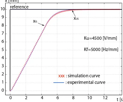
Finally, we use reasonable values ofKUandKf. The simulation and experimental results are shown in Figure 1.22. First, the speed is constant (case a) because both the amplitude and the frequency are saturated. Atxf s = fs/Kf, the frequency leaves the saturation but not the amplitude. This corresponds to the frequency proportional controller presented in case d. According to the values ofKU andKf, the amplitude saturation may occur instead of the frequency saturation. From xU S =Us/KU, the voltage is no longer saturated and case e occurs. Hence, the static error is given by εstat=U0/KU.

1.7. Conclusion

(38)

0 2 4 6 8 _{10 t [s]}

xxx : simulation result : experimental result

Figure 1.21.(a) LowKUand highKf and (b) highKUand lowKf

et Technologie(FEMTO-ST) Institute in the AS2M department, has been discussed. Based on the use of piezoelectric actuators, this device can be operated either in coarse mode or in sub-step mode.

In the sub-step mode, the legs never slide and the obtained accuracy is 5 nm. This mode is suitable when the difference between the reference position and the current position is less than 1 step.

(39)

0 2 4 6 8 10 12 _{t [s]} x [mm]

xfS

xUS

xxx : simulation curve : experimental curve

0 1 2 3 4 5 6 7 8 9 10

Ku=4500 [V/mm]

Kf=5000 [Hz/mm] reference

Figure 1.22.Acceptable values ofKUandKf

of the controller has been proven. The performances of the coarse mode are given by the hardware performances. Combining the sub-step mode and the coarse mode is a solution for performing high-stroke/high-precision positioning tasks. The coarse mode will be used to drive the device close to the reference position and the sub-step mode will provide additional displacement details required to reach the reference. However, this approach requires the use of a long-range/high-accuracy position sensor, which is not easy to integrate. This will be an area of future research.

1.8. Bibliography

[ARM 94] ARMSTRONG-HÉLOUVRYB., DUPONTP., CANUDAS-DE-WIT C., “A survey of models, analysis tools and compensation methods for the control of machines with friction”, IFAC Automatica, vol. 30, num. 7, p. 1083–1138, 1994. [BER 03] BERGANDER A., DRIESEN W., VARIDEL T., BREGUET J. M.,

“Mono-lithic piezoelectric push-pull actuators for inertial drives”, IEEE International Symposium on Micromechatronics and Human Science, p. 309–316, 2003. [BER 04] BERGANDER A., DRIESEN W., VARIDEL T., MEIZOSO M., BREGUET

J., “Mobile cm3-microrobots with tools for nanoscale imaging and micromanipu-lation”,Proceedings of IEEE International Symposium on Micromechatronics and Human Science (MHS), Nagoya, Japan, p. 309–316, 2004.

(40)

[BRE 98] BREGUETJ., CLAVELR., “Stick and slip actuators: design, control, perfor-mances and applications”, IEEE International Symposium on Micromechatronics and Human Science, p. 89–95, 1998.

[DRI 03] DRIESEN W., BERGANDER A., VARIDEL T., BREGUET J., “Energy consumption of piezoelectric actuators for inertial drives”, IEEE International Symposium on Micromechatronics and Human Science, p. 51–58, 2003.

[DUP 02] DUPONTP., HAYWARDV., ARMSTRONGB., ALTPETERF., “Single state elastoplastic friction models”, IEEE Transactions on Automatic Control, vol. 47, num. 5, p. 787–792, 2002.

[FAT 95] FATIKOW S., MAGNUSSEN B., REMBOLD U., “A piezoelectric mobile robot for handling of micro-objects”, Proceedings of the International Symposium on Microsystems, Intelligent Materials and Robots, p. 189–192, 1995.

[GAR 00] GARTNERC., BLUMELV., KRAPLINA., POSSNERT., “Micro-assembly processes for beam transformation systems of high-power laser diode bars”, MST news I, p. 23–24, 2000.

[RAK 06] RAKOTONDRABE M., Design, development and modular control of a microassembly station, PhD thesis, University of Franche-Comté, 2006.

[RAK 08] RAKOTONDRABE M., HADDAB Y., LUTZ P., “Voltage/frequency proportional control of stick-slip micropositioning systems”, IEEE Transactions on Control Systems Technology, vol. 16, num. 6, p. 1316–1322, 2008.

[RAK 09] RAKOTONDRABE M., HADDAB Y., LUTZ P., “Development, sub-step modelling and control of a micro/nano positioning 2DoF stick-slip device”, IEEE/ASME Transactions on Mechatronics, 2009, DOI 10.1109/TMECH.2009.2011134.

(41)

Microbeam Dynamic Shaping by Closed-loop

Electrostatic Actuation using Modal Control

A contribution to flexible microstructure control is developed in this chapter using large arrays of nanotransducers. The distributed transduction scheme consists of two sets ofNelectrodes located on each side of the microstructure for electrostatic driving and capacitive detection. Since accurate point-to-point control requires a large number of controllers, modal control is proposed to limit integration complexity. This is carried out by projecting the measured displacements on then(<< N) modes to be controlled before calculating the stresses that must be distributed throughout the beam. Although simple PID control can be used, fabrication tolerances, parameter variations and model simplifications require robust specifications ensured by sophisticated control laws. An example of the combination of the Loop Transfer Recovery (LTR) method with the Full State Feedback (FSF) control extended standard models is presented, showing high robust stability and performances.

2.1. Introduction

Smart materials and intelligent structures are a new rapidly growing technology embracing the fields of sensor and actuator systems, information processing and control. They are capable of sensing and reacting to their environment in a predictable and desired manner and are used to carry mechanical loads, alleviate vibration, reduce acoustic noise, monitor their own condition and environment, automatically perform precision alignments or change their shape or mechanical properties on command.

(42)

While active structural control may be described as seeking a distributed control actuation such that a desired spatial distribution of the structure displacement is reached, in dynamic shape control the desired shape has to be additionally prescribed as a function of time.

In astronomical sciences, adaptive optical elements such as deformable mirrors used to correct for atmospheric aberrations provide a good example of shape control structures [LIA 97, ROO 02]. As the high cost of piezoelectric actuated mirrors prevented the broader adoption of this technology, deformable mirrors based on microelectromechanical systems (MEMS) have recently emerged [KEN 07]. These micromirrors are less costly and have enabled many new applications in bio-imaging including retina imaging, optical coherence tomography and wide-field microscopy. They were first used by [DRE 89] for a membrane mirror with 13 actuators in a scanning laser ophthalmoscope. More recently, adaptive aberration correction was investigated using membrane mirrors having 37 actuators [FER 03], while retinal images were obtained by a 140-actuator micromachined mirror [DOB 02].

It is highly desirable to suppress residual vibrations introduced in the mechanical structures by high-speed scanning motion and flexure actuation [POP 04]. In this context, the zero-vibration derivative method introduced by Singer and Seering [SIN 89] is well known. Other input-shaping work using a model-matching technique [POP 03] makes it possible to enforce realistic input and state constraints. This time-domain model-matching method is also used in [POP 04] to address the inverse control problem without using sensors for feedback. Moreover, other performances are required such as minimizing overshoot or following a certain motion profile. In optical switching systems, for example, the point-to-point motion of micromirrors used for redirecting optical signals has to be controlled. Typical settling times are of the order of a few milliseconds [CHI 00].

In recent years, a new MEMS actuation-sensing paradigm has been applied to control microstructures, particularly in aerospace and the automotive industry where microactuators, multistable relays, microconnectors and micropropulsion systems are used. Since fabrication technologies and processes have been developed and implemented, MEMS microstructures must be integrated with signal processing and controlling ICs and controllers must be designed [JUD 97, HO 98, LYS 99]. Point-to-point actuation and sensing performed by microstructures are not sufficient in such advanced applications. The real-time intelligent coordinated motion of microstructure arrays, a very challenging problem, is required to guarantee the desired surface deflections and geometries [LYS 01].

(43)

within the microdevices (actuators–sensors) through power, communication and control channels. The complexity of distributed systems is therefore greater than the complexity of centralized control systems [LYS 02].

Actuation mechanisms for MEMS vary depending on the suitability to the particular application. The most common actuation mechanisms are electrostatic, pneumatic, thermal and piezoelectric; electrostatic actuation is one of the most common principles in the field of MEMS [ABD 05], from simple RF microswitches [PAR 01] to high-precision adaptive micromirrors [VDO 01]. This is due to its simplicity, since it requires few mechanical components, and small voltage levels for actuation.

The structural elements that are used in MEMS devices are typically simple elements such as beams, plates and membranes. However, the fact that the pressure– voltage and displacement–pressure relationships are non-linear makes such MEMS very difficult to design accurately: the mechanical part of the device is most often described by linear models or simple non-linear models [WAN 96, DUF 99]. Some approaches to the design of electrostatic microactuators include: [HIS 93] in which a micromirror is fabricated with a three-dimensional (3D) thickness profile and allows an optically ideal deformation; and [HUN 98] in which the shape of an electrode is changed to achieve a particular voltage–capacitance relationship.

In [COL 05], the authors describe a method for calculating the voltage distribution necessary to achieve a given shape. They solve the non-linear mechanical inverse problem to calculate the ideal pressure distribution and then solve the quadratic programming problem to find the voltages that give the best approximation to this ideal pressure distribution. At the same time, piezoelectric (PZT) actuators have long been used in lightweight adaptive optics.

In [LIU 93] and [HUO 97], PZT actuators were bonded in optical mirrors to achieve designed surface shapes. Recently, as dynamic shape tracking has gained attention as well as integrating structural shape control and motion control, dynamic displacement tracking of smart beams has been studied using distributed self-stress/strain sensors and actuators [KRO 07] or piezoelectric types [IRS 02, IRS 06]. A sequential linear least-squares algorithm (SLLS) for tracking the dynamic shapes of PZT smart structures is formulated in [LUO 06]. In [LUO 07], an efficient algorithm for dynamic shape tracking with optimum energy control is proposed. [KAD 03] present an implementation of distributed optimal control strategy that limits the required data to only adjacent sensors.

(44)

important computational time and algorithms as well as complex controller networks remain the main problems of distributed active MEMS control.

In this chapter, we describe an automatic mode-based control method applied to electrostatically driven microstructures in order to accurately track a dynamic shape reference with fast time response, high robustness against parameter uncertainty and measurement noise reduction. A modal analysis describes the structure displacement shape by a few modal components that are to be controlled instead of the point-to-point control. This technique allows the number of required controllers to be reduced, especially when many transducers are used. Control design is carried out using two approaches: proportional integral derivative (PID) control and full state feedback (FSF) control. The main advantage of the former lies in the simplicity of its design and implementation, while the latter is superior in terms of robustness properties.

2.2. System description

Smart structures used in the literature are of several types and geometrical shape. The most popular are cantilevers, clamped-clamped beams and membranes. Since electrostatic actuation has the merits of low power consumption, simple driving electronics and ease of fabrication and integration, it has become one of the most popular driving methods; it offers integrated detection without the need for an additional position sensing device. In the example discussed in this chapter, a continuous deformable microbeam clamped on both extremities is considered. Two sets of N nanoelectrodes are disposed on both sides of the microbeam forming distributed electrode-to-structure capacitors that act as electromechanical transducers, transferring the energy between the electrical and mechanical domains (actuation and detection means). A view of the system is depicted in Figure 2.1.

Figure 2.1.Schematic view of the system

(45)

electrode direction. For each positionxi, depending on the calculated control signal, the voltage is applied to one of the two electrodes on either side according to the sign of the required force. The commutation of the drive electrodes is accomplished by a multiplexing system as depicted in Figure 2.1. The first-order approximate relation expressing the electrostatic force on positionxias a function of the electrode voltage Viapplied to the corresponding electrode is:

f(xi, t) = ǫ0SeV

2 i

2(g−w(xi, t))2 (2.1)

where Se is the area of the electrode, ǫ0 is the permittivity in vacuum, g is the initial gap between the microbeam and the electrode andw(xi, t)is the transverse displacement of the microbeam at position xi. The latter is measured by capacitive means which consists of detecting an output current, dependent upon the electrode-to-resonator capacitance, as a function of the microbeam displacement. The first-order approximate equation expressing this capacitance to the displacement is

C(xi, t) = ǫ0Se

2(g−w(xi, t)). (2.2)

In previous research, actuation and capacitive sensing are implemented through separate physical structures [CHA 95, HOR 00, KUI 04] which increase the overall size of the device, modify its mechanical characteristics and add flexural structures that reduce the displacement range of the system. It is therefore more advantageous to use the same capacitive structure for both actuation and sensing purposes.

When tracking static deformations or low-frequency dynamical shapes, the capac-itive detection becomes more problematic because no current flow is obtained for low or null frequencies. However, since the mechanical device behaves as a superposition of modal low-pass filters (as described in the next section), a low input signal with frequency orders of magnitude higher than the mechanical modal frequencies can be used as a sensing signal without evoking mechanical response. Electrically, this sensing signal experiences amplitude and phase modulation due to the capacitance change of the drive (function of the mechanical displacement). By monitoring it, a measure of the displacement is inferred [DON 08]. Figure 2.2 shows the displacement measurement scheme of simultaneous actuating/sensing capacitive drives.

(46)

Figure 2.2.Displacement measurement scheme on simultaneous actuating/detection capacitive drives

many electrodes adds to the complexity of fabrication, miniaturization and control computation for the point-by-point classical control methods.

2.3. Modal analysis

The out-of-plane time-dependent transverse displacement w(x, t) of the micro-beam at every positionxis governed by the Euler–Bernoulli equation. By considering a beam of lengthl, thicknesseand widthh, we can describe its deformation behavior when subjected to an external distributed strengthf(x, t)by:

EI∂

4_w₍_{x, t}₎

∂x4 +T(w(x, t))

∂2_w₍_{x, t}₎ ∂x2 +b

∂w(x, t)

∂t +ρS

∂2_w₍_{x, t}₎

∂t2 =f(x, t) (2.3) where S = he is the transversal section of the beam, E is Young’s modulus, I = e3_h/₁₂ _{is the moment of inertia,} _ρ_{is density,} _b _{is the friction coefficient of} interaction with the surrounding fluid andT(w(x, t))is the stress associated with the beam elongation.

We associate boundary conditions of the structure with equation (2.3). Most often, in the MEMS field, the boundary conditions are defined by one of the two states:

– free edge:w′′

=w′′′

= 0, – clamped edge:w=w′

= 0.

A schematic 3D representation of the clamped-clamped microbeam is shown in Figure 2.3.

A solution of equation (2.3) can be found by decomposing w(x, t) on the eigenmodes of the operator∂4_/∂x4_{, that is}

w(x, t) =

n

k=1

(47)

Figure 2.3.Clamped-clamped microbeam illustrating the dimension variablesl_,e_andh

and where wk(x) are the n eigenvectors (also called mode shape vectors), λ4 k are the corresponding eigenvalues and ak(t)are the dynamic corresponding modal coefficients.

A solution of equation (2.5) is

wk =Acos(λkx) +Bsin(λkx) +Ccosh(λkx) +Dsinh(λkx) (2.6)

where A, B, C and D are four constants that depend on the boundary conditions. Considering our clamped-clamped case, we have

⎧

(48)

The eigenvectorswk(x)become

and form an orthogonal basis for the scalar product

u|v=

l

0

u(x)v(x)dx. (2.11)

To obtain an orthormal basis,Akis chosen such that

Ak=

Considering equations (2.4) and (2.5), equation (2.3) can be written as

n

wherefk are the components of the distributed force on each modek. Note that the beam elongationT(w)is independent of the positionx.

Figure 2.4 shows the modal shapes of the five first modes of a clamped-clamped microbeam of lengthl= 5µm.

Projecting equation (2.13) on each eigenvectorwi (i = 1 → n), taking into consideration the orthogonality of the basis, yieldsNequations of the form

EIaiλ4i +T(w)

Thesenequations represent the equations of motion of theNmodal coefficientsai in relation to their corresponding force modal componentfi, and they can be written in a matrix form as

(49)

0 100 0

Figure 2.4.First five modal shapes of the clamped-clamped microbeam

where

The stress due to the small elongation∆lof the microbeam is expressed as

(50)

which gives

the stress can be described in a matrix representation as

T(w) = −ES

2l X

T_AX _(2.20)

leading to the non-linear term

N(X) =−ES

As mentioned in section 2.1, smart structures are usually used to track a reference shape or deformation which can be represented by a set of reference displacements along the microstructure surface. This reference can be static or dynamic (or null in the case of vibrations suppression).

For the microbeam example described in section 2.2, the reference shape is described by a 1D vector of N displacements onN positions along the microbeam length corresponding to the centers of the actuating/sensing electrodes. In the literature, many MEMS devices are typically driven in an open-loop fashion by applying simple input control signals. Modifying and improving the mechanical design of MEMS actuators have resulted in more suitable straightforward driving signals. Pre-shaped control is also adopted to achieve better dynamical performance when knowledge of system dynamics is available. However, the lack of accurate models, fabrication inconsistencies, parameter variation, external disturbances and dynamical behavior specifications call for the use of closed-loop control design.

(51)

One solution to this problem is to control only the dynamic modal coefficients instead of the direct displacements. The number of the required controllers will therefore be limited to a few modes independently of the actuators number. The numbernof the controlled modes is fixed by the required reference shapes considered (in our case) as a linear combination of the five first modes, believed to comprise sufficient deformation shapes for one microbeam. When regulating allak(t)to their reference values ¯ak(t)for k = 1 → n, the shape deformationw(xi, t)tracks the referencew¯(xi, t) =n

1¯ak(t)wk(xi).

The architecture of the closed-loop system using modal control is depicted in Figure 2.5.

Figure 2.5.Closed-loop system using modal control

By using modal control, we will be dealing with the modal equations of motion represented in equation (2.15), avoiding the (equation (2.3)) non-linear coupled point-to-point displacements. These modal equations of motion are assumed to be linear for small displacements, neglecting the modes-coupling term resulting from elongation stresses. In this case, the equations in matrix equation (2.15) describe the behavior ofn linear uncoupled second-order mass-spring-damping systems with known parameters of stiffness, mass and damping coefficient. Hence, shape tracking dynamics can be fixed by control.

Basically, two types of time-varying functions for smart structure deflections are considered: the triangular and the sinusoidal [LUO 06, LUO 07]. In this chapter, two methods of control design are adopted: PID control based on the tracking errors and FSF control based on all the states of a so-called ‘standard model’. In both approaches, displacement measures are projected on the five modes to obtain the modal coefficients ak(t)and controller outputs are expressed by modal force coefficientsfk(t), used to recompose the required distributed force to be applied to the microbeam:

f(xi, t) =

n

k=1