Mathematics for Finance:
An Introduction to
Financial Engineering
Marek Capinski
Tomasz Zastawniak
Springer Undergraduate Mathematics Series
Advisory Board
P.J. Cameron Queen Mary and Westfield College
M.A.J. Chaplain University of Dundee
K. Erdmann Oxford University
L.C.G. Rogers University of Cambridge
E. Süli Oxford University
J.F. Toland University of Bath
Other books in this series
A First Course in Discrete Mathematics I. Anderson
Analytic Methods for Partial Differential Equations G. Evans, J. Blackledge, P. Yardley
Applied Geometry for Computer Graphics and CAD D. Marsh
Basic Linear Algebra, Second Edition T.S. Blyth and E.F. Robertson
Basic Stochastic Processes Z. Brze´zniak and T. Zastawniak
Elementary Differential Geometry A. Pressley
Elementary Number Theory G.A. Jones and J.M. Jones Elements of Abstract Analysis M. Ó Searcóid
Elements of Logic via Numbers and Sets D.L. Johnson Essential Mathematical Biology N.F. Britton
Fields, Flows and Waves: An Introduction to Continuum Models D.F. Parker
Further Linear Algebra T.S. Blyth and E.F. Robertson
Geometry R. Fenn
Groups, Rings and Fields D.A.R. Wallace
Hyperbolic Geometry J.W. Anderson
Information and Coding Theory G.A. Jones and J.M. Jones
Introduction to Laplace Transforms and Fourier Series P.P.G. Dyke
Introduction to Ring Theory P.M. Cohn
Introductory Mathematics: Algebra and Analysis G. Smith
Linear Functional Analysis B.P. Rynne and M.A. Youngson
Matrix Groups: An Introduction to Lie Group Theory A. Baker
Measure, Integral and Probability M. Capi´nski and E. Kopp
Multivariate Calculus and Geometry S. Dineen
Numerical Methods for Partial Differential Equations G. Evans, J. Blackledge, P. Yardley
Probability Models J. Haigh
Real Analysis J.M. Howie
Sets, Logic and Categories P. Cameron
Special Relativity N.M.J. Woodhouse
Symmetries D.L. Johnson
Topics in Group Theory G. Smith and O. Tabachnikova
Topologies and Uniformities I.M. James
Marek Capi´nski and Tomasz Zastawniak
Mathematics for
Finance
An Introduction to Financial Engineering
With 75 Figures
Marek Capi´nski
Nowy Sacz School of Business–National Louis University, 33-300 Nowy Sacz, ul. Zielona 27, Poland
Tomasz Zastawniak
Department of Mathematics, University of Hull, Cottingham Road, Kingston upon Hull, HU6 7RX, UK
Cover illustration elements reproduced by kind permission of:
Aptech Systems, Inc., Publishers of the GAUSS Mathematical and Statistical System, 23804 S.E. Kent-Kangley Road, Maple Valley, WA 98038, USA. Tel: (206) 432 - 7855 Fax (206) 432 - 7832 email: [email protected] URL: www.aptech.com.
American Statistical Association: Chance Vol 8 No 1, 1995 article by KS and KW Heiner ‘Tree Rings of the Northern Shawangunks’ page 32 fig 2.
Springer-Verlag: Mathematica in Education and Research Vol 4 Issue 3 1995 article by Roman E Maeder, Beatrice Amrhein and Oliver Gloor ‘Illustrated Mathematics: Visualization of Mathematical Objects’ page 9 fig 11, originally published as a CD ROM ‘Illustrated Mathematics’ by TELOS: ISBN 0-387-14222-3, German edition by Birkhauser: ISBN 3-7643-5100-4.
Mathematica in Education and Research Vol 4 Issue 3 1995 article by Richard J Gaylord and Kazume Nishidate ‘Traffic Engineering with Cellular Automata’ page 35 fig 2. Mathematica in Education and Research Vol 5 Issue 2 1996 article by Michael Trott ‘The Implicitization of a Trefoil Knot’ page 14.
Mathematica in Education and Research Vol 5 Issue 2 1996 article by Lee de Cola ‘Coins, Trees, Bars and Bells: Simulation of the Binomial Process’ page 19 fig 3. Mathematica in Education and Research Vol 5 Issue 2 1996 article by Richard Gaylord and Kazume Nishidate ‘Contagious Spreading’ page 33 fig 1. Mathematica in Education and Research Vol 5 Issue 2 1996 article by Joe Buhler and Stan Wagon ‘Secrets of theMadelung Constant’ page 50 fig 1.
British Library Cataloguing in Publication Data Capi´nski, Marek,
1951-Mathematics for finance : an introduction to financial engineering. - (Springer undergraduate mathematics series) 1. Business mathematics 2. Finance – Mathematical models I. Title II. Zastawniak, Tomasz,
1959-332’.0151 ISBN 1852333308
Library of Congress Cataloging-in-Publication Data Capi´nski, Marek,
1951-Mathematics for finance : an introduction to financial engineering / Marek Capi´nskiand
Tomasz Zastawniak.
p. cm. — (Springer undergraduate mathematics series) Includes bibliographical references and index.
ISBN 1-85233-330-8 (alk. paper)
1. Finance – Mathematical models. 2. Investments – Mathematics. 3. Business mathematics. I. Zastawniak, Tomasz, 1959- II. Title. III. Series.
HG106.C36 2003
332.6’01’51—dc21 2003045431
Apart from any fair dealing for the purposes of research or private study, or criticism or review, as permitted under the Copyright, Designs and Patents Act 1988, this publication may only be reproduced, stored or transmitted, in any form or by any means, with the prior permission in writing of the publishers, or in the case of reprographic reproduction in accordance with the terms of licences issued by the Copyright Licensing Agency. Enquiries concerning reproduction outside those terms should be sent to the publishers.
Springer Undergraduate Mathematics Series ISSN 1615-2085 ISBN 1-85233-330-8 Springer-Verlag London Berlin Heidelberg
a member of BertelsmannSpringer Science+Business Media GmbH http://www.springer.co.uk
© Springer-Verlag London Limited 2003 Printed in the United States of America
The use of registered names, trademarks etc. in this publication does not imply, even in the absence of a specific statement, that such names are exempt from the relevant laws and regulations and therefore free for general use.
The publisher makes no representation, express or implied, with regard to the accuracy of the information contained in this book and cannot accept any legal responsibility or liability for any errors or omissions that may be made.
Typesetting: Camera ready by the authors
Preface
True to its title, this book itself is an excellent financial investment. For the price of one volume it teaches two Nobel Prize winning theories, with plenty more included for good measure. How many undergraduate mathematics textbooks can boast such a claim?
Building on mathematical models of bond and stock prices, these two theo-ries lead in different directions: Black–Scholes arbitrage pricing of options and other derivative securities on the one hand, and Markowitz portfolio optimisa-tion and the Capital Asset Pricing Model on the other hand. Models based on the principle of no arbitrage can also be developed to study interest rates and their term structure. These are three major areas of mathematical finance, all having an enormous impact on the way modern financial markets operate. This textbook presents them at a level aimed at second or third year undergraduate students, not only of mathematics but also, for example, business management, finance or economics.
The contents can be covered in a one-year course of about 100 class hours. Smaller courses on selected topics can readily be designed by choosing the appropriate chapters. The text is interspersed with a multitude of worked ex-amples and exercises, complete with solutions, providing ample material for tutorials as well as making the book ideal for self-study.
Prerequisites include elementary calculus, probability and some linear alge-bra. In calculus we assume experience with derivatives and partial derivatives, finding maxima or minima of differentiable functions of one or more variables, Lagrange multipliers, the Taylor formula and integrals. Topics in probability include random variables and probability distributions, in particular the bi-nomial and normal distributions, expectation, variance and covariance, condi-tional probability and independence. Familiarity with the Central Limit The-orem would be a bonus. In linear algebra the reader should be able to solve
vi Mathematics for Finance
systems of linear equations, add, multiply, transpose and invert matrices, and compute determinants. In particular, as a reference in probability theory we recommend our book: M. Capi´nski and T. Zastawniak, Probability Through Problems, Springer-Verlag, New York, 2001.
In many numerical examples and exercises it may be helpful to use a com-puter with a spreadsheet application, though this is not absolutely essential. Microsoft Excel files with solutions to selected examples and exercises are avail-able on our web page at the addresses below.
We are indebted to Nigel Cutland for prompting us to steer clear of an inaccuracy frequently encountered in other texts, of which more will be said in Remark 4.1. It is also a great pleasure to thank our students and colleagues for their feedback on preliminary versions of various chapters.
Readers of this book are cordially invited to visit the web page below to check for the latest downloads and corrections, or to contact the authors. Your comments will be greatly appreciated.
Marek Capi´nski and Tomasz Zastawniak January 2003
Contents
1. Introduction: A Simple Market Model. . . 1
1.1 Basic Notions and Assumptions . . . 1
1.2 No-Arbitrage Principle . . . 5
1.3 One-Step Binomial Model . . . 7
1.4 Risk and Return . . . 9
1.5 Forward Contracts . . . 11
1.6 Call and Put Options . . . 13
1.7 Managing Risk with Options . . . 19
2. Risk-Free Assets. . . 21
2.1 Time Value of Money . . . 21
2.1.1 Simple Interest . . . 22
2.1.2 Periodic Compounding . . . 24
2.1.3 Streams of Payments . . . 29
2.1.4 Continuous Compounding . . . 32
2.1.5 How to Compare Compounding Methods . . . 35
2.2 Money Market . . . 39
2.2.1 Zero-Coupon Bonds . . . 39
2.2.2 Coupon Bonds . . . 41
2.2.3 Money Market Account . . . 43
3. Risky Assets. . . 47
3.1 Dynamics of Stock Prices . . . 47
3.1.1 Return . . . 49
3.1.2 Expected Return . . . 53
3.2 Binomial Tree Model . . . 55
viii Contents
3.2.1 Risk-Neutral Probability . . . 58
3.2.2 Martingale Property . . . 61
3.3 Other Models . . . 63
3.3.1 Trinomial Tree Model . . . 64
3.3.2 Continuous-Time Limit . . . 66
4. Discrete Time Market Models . . . 73
4.1 Stock and Money Market Models . . . 73
4.1.1 Investment Strategies . . . 75
4.1.2 The Principle of No Arbitrage . . . 79
4.1.3 Application to the Binomial Tree Model . . . 81
4.1.4 Fundamental Theorem of Asset Pricing . . . 83
4.2 Extended Models . . . 85
5. Portfolio Management. . . 91
5.1 Risk . . . 91
5.2 Two Securities . . . 94
5.2.1 Risk and Expected Return on a Portfolio . . . 97
5.3 Several Securities . . . 107
5.3.1 Risk and Expected Return on a Portfolio . . . 107
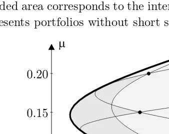
5.3.2 Efficient Frontier . . . 114
5.4 Capital Asset Pricing Model . . . 118
5.4.1 Capital Market Line . . . 118
5.4.2 Beta Factor . . . 120
5.4.3 Security Market Line . . . 122
6. Forward and Futures Contracts. . . .125
6.1 Forward Contracts . . . 125
6.1.1 Forward Price . . . 126
6.1.2 Value of a Forward Contract . . . 132
6.2 Futures . . . 134
6.2.1 Pricing . . . 136
6.2.2 Hedging with Futures . . . 138
7. Options: General Properties. . . .147
7.1 Definitions . . . 147
7.2 Put-Call Parity . . . 150
7.3 Bounds on Option Prices . . . 154
7.3.1 European Options . . . 155
7.3.2 European and American Calls on Non-Dividend Paying Stock . . . 157
Contents ix
7.4 Variables Determining Option Prices . . . 159
7.4.1 European Options . . . 160
7.4.2 American Options . . . 165
7.5 Time Value of Options . . . 169
8. Option Pricing. . . .173
8.1 European Options in the Binomial Tree Model . . . 174
8.1.1 One Step . . . 174
8.1.2 Two Steps . . . 176
8.1.3 General N-Step Model . . . 178
8.1.4 Cox–Ross–Rubinstein Formula . . . 180
8.2 American Options in the Binomial Tree Model . . . 181
8.3 Black–Scholes Formula . . . 185
9. Financial Engineering. . . .191
9.1 Hedging Option Positions . . . 192
9.1.1 Delta Hedging . . . 192
9.1.2 Greek Parameters . . . 197
9.1.3 Applications . . . 199
9.2 Hedging Business Risk . . . 201
9.2.1 Value at Risk . . . 202
9.2.2 Case Study . . . 203
9.3 Speculating with Derivatives . . . 208
9.3.1 Tools . . . 208
9.3.2 Case Study . . . 209
10. Variable Interest Rates . . . .215
10.1 Maturity-Independent Yields . . . 216
10.1.1 Investment in Single Bonds . . . 217
10.1.2 Duration . . . 222
10.1.3 Portfolios of Bonds . . . 224
10.1.4 Dynamic Hedging . . . 226
10.2 General Term Structure . . . 229
10.2.1 Forward Rates . . . 231
10.2.2 Money Market Account . . . 235
11. Stochastic Interest Rates . . . .237
11.1 Binomial Tree Model . . . 238
11.2 Arbitrage Pricing of Bonds . . . 245
11.2.1 Risk-Neutral Probabilities . . . 249
11.3 Interest Rate Derivative Securities . . . 253
x Contents
11.3.2 Swaps . . . 255
11.3.3 Caps and Floors . . . 258
11.4 Final Remarks . . . 259
Solutions . . . .263
Bibliography. . . .303
Glossary of Symbols. . . .305
1
Introduction: A Simple Market Model
1.1 Basic Notions and Assumptions
Suppose that two assets are traded: one risk-free and one risky security. The former can be thought of as a bank deposit or a bond issued by a government, a financial institution, or a company. The risky security will typically be some stock. It may also be a foreign currency, gold, a commodity or virtually any asset whose future price is unknown today.
Throughout the introduction we restrict the time scale to two instants only: today,t= 0, and some future time, say one year from now,t= 1. More refined and realistic situations will be studied in later chapters.
The position in risky securities can be specified as the number of shares of stock held by an investor. The price of one share at timet will be denoted byS(t). The current stock priceS(0) is known to all investors, but the future price S(1) remains uncertain: it may go up as well as down. The difference
S(1)−S(0) as a fraction of the initial value represents the so-called rate of return, or brieflyreturn:
KS =
S(1)−S(0)
S(0) ,
which is also uncertain. The dynamics of stock prices will be discussed in Chap-ter 3.
The risk-free position can be described as the amount held in a bank ac-count. As an alternative to keeping money in a bank, investors may choose to invest in bonds. The price of one bond at timet will be denoted byA(t). The
2 Mathematics for Finance
current bond price A(0) is known to all investors, just like the current stock price. However, in contrast to stock, the priceA(1) the bond will fetch at time 1 is also known with certainty. For example,A(1) may be a payment guaranteed by the institution issuing bonds, in which case the bond is said to mature at time 1 with face valueA(1). The return on bonds is defined in a similar way as that on stock,
KA=
A(1)−A(0)
A(0) .
Chapters 2, 10 and 11 give a detailed exposition of risk-free assets.
Our task is to build a mathematical model of a market of financial securi-ties. A crucial first stage is concerned with the properties of the mathematical objects involved. This is done below by specifying a number of assumptions, the purpose of which is to find a compromise between the complexity of the real world and the limitations and simplifications of a mathematical model, imposed in order to make it tractable. The assumptions reflect our current position on this compromise and will be modified in the future.
Assumption 1.1 (Randomness)
The future stock price S(1) is a random variable with at least two different values. The future priceA(1) of the risk-free security is a known number.
Assumption 1.2 (Positivity of Prices)
All stock and bond prices are strictly positive,
A(t)>0 and S(t)>0 fort= 0,1.
The total wealth of an investor holding x stock shares and y bonds at a time instantt= 0,1 is
V(t) =xS(t) +yA(t).
The pair (x, y) is called aportfolio,V(t) being thevalue of this portfolio or, in other words, thewealth of the investor at timet.
The jumps of asset prices between times 0 and 1 give rise to a change of the portfolio value:
V(1)−V(0) =x(S(1)−S(0)) +y(A(1)−A(0)).
This difference (which may be positive, zero, or negative) as a fraction of the initial value represents the return on the portfolio,
KV =
V(1)−V(0)
1. Introduction: A Simple Market Model 3
The returns on bonds or stock are particular cases of the return on a portfolio (with x = 0 or y = 0, respectively). Note that because S(1) is a random variable, so is V(1) as well as the corresponding returns KS and KV. The
returnKA on a risk-free investment is deterministic.
Example 1.1
LetA(0) = 100 and A(1) = 110 dollars. Then the return on an investment in bonds will be
KA= 0.10,
that is, 10%. Also, letS(0) = 50 dollars and suppose that the random variable
S(1) can take two values,
S(1) =
52 with probabilityp, 48 with probability 1−p, for a certain 0< p <1. The return on stock will then be
KS =
0.04 if stock goes up,
−0.04 if stock goes down, that is, 4% or−4%.
Example 1.2
Given the bond and stock prices in Example 1.1, the value at time 0 of a portfolio withx= 20 stock shares and y= 10 bonds is
V(0) = 2,000
dollars. The time 1 value of this portfolio will be
V(1) =
2,140 if stock goes up, 2,060 if stock goes down,
so the return on the portfolio will be
KV =
0.07 if stock goes up, 0.03 if stock goes down,
4 Mathematics for Finance
Exercise 1.1
LetA(0) = 90,A(1) = 100,S(0) = 25 dollars and let
S(1) =
30 with probabilityp, 20 with probability 1−p,
where 0< p <1. For a portfolio withx= 10 shares and y= 15 bonds calculateV(0),V(1) andKV.
Exercise 1.2
Given the same bond and stock prices as in Exercise 1.1, find a portfolio whose value at time 1 is
V(1) =
1,160 if stock goes up, 1,040 if stock goes down.
What is the value of this portfolio at time 0?
It is mathematically convenient and not too far from reality to allow arbi-trary real numbers, including negative ones and fractions, to represent the risky and risk-free positionsxandy in a portfolio. This is reflected in the following assumption, which imposes no restrictions as far as the trading positions are concerned.
Assumption 1.3 (Divisibility, Liquidity and Short Selling)
An investor may hold any numberxandyof stock shares and bonds, whether integer or fractional, negative, positive or zero. In general,
x, y∈R.
The fact that one can hold a fraction of a share or bond is referred to as divisibility. Almost perfect divisibility is achieved in real world dealings whenever the volume of transactions is large as compared to the unit prices.
The fact that no bounds are imposed onxoryis related to another market attribute known asliquidity. It means that any asset can be bought or sold on demand at the market price in arbitrary quantities. This is clearly a mathe-matical idealisation because in practice there exist restrictions on the volume of trading.
1. Introduction: A Simple Market Model 5
securities may involve issuing and selling bonds, but in practice the same fi-nancial effect is more easily achieved by borrowing cash, the interest rate being determined by the bond prices. Repaying the loan with interest is referred to asclosing the short position. A short position in stock can be realised byshort selling. This means that the investor borrows the stock, sells it, and uses the proceeds to make some other investment. The owner of the stock keeps all the rights to it. In particular, she is entitled to receive any dividends due and may wish to sell the stock at any time. Because of this, the investor must always have sufficient resources to fulfil the resulting obligations and, in particular, to close the short position in risky assets, that is, to repurchase the stock and return it to the owner. Similarly, the investor must always be able to close a short position in risk-free securities, by repaying the cash loan with interest. In view of this, we impose the following restriction.
Assumption 1.4 (Solvency)
The wealth of an investor must be non-negative at all times,
V(t)≥0 fort= 0,1.
A portfolio satisfying this condition is calledadmissible.
In the real world the number of possible different prices is finite because they are quoted to within a specified number of decimal places and because there is only a certain final amount of money in the whole world, supplying an upper bound for all prices.
Assumption 1.5 (Discrete Unit Prices)
The future price S(1) of a share of stock is a random variable taking only finitely many values.
1.2 No-Arbitrage Principle
In this section we are going to state the most fundamental assumption about the market. In brief, we shall assume that the market does not allow for risk-free profits with no initial investment.
6 Mathematics for Finance
while dealerB in London sells them at a rate dB = 1.60 dollars to a pound.
If this were the case, the dealers would, in effect, be handing out free money. An investor with no initial capital could realise a profit of dA −dB = 0.02
dollars per each pound traded by taking simultaneously a short position with dealer B and a long position with dealer A. The demand for their generous services would quickly compel the dealers to adjust the exchange rates so that this profitable opportunity would disappear.
Exercise 1.3
On 19 July 2002 dealerAin New York and dealerBin London used the following rates to change currency, namely euros (EUR), British pounds (GBP) and US dollars (USD):
dealerA buy sell
1.0000 EUR 1.0202 USD 1.0284 USD 1.0000 GBP 1.5718 USD 1.5844 USD
dealerB buy sell
1.0000 EUR 0.6324 GBP 0.6401 GBP 1.0000 USD 0.6299 GBP 0.6375 GBP
Spot a chance of a risk-free profit without initial investment.
The next example illustrates a situation when a risk-free profit could be realised without initial investment in our simplified framework of a single time step.
Example 1.3
Suppose that dealerA in New York offers to buy British pounds a year from now at a ratedA= 1.58 dollars to a pound, while dealerBin London would sell
British pounds immediately at a ratedB = 1.60 dollars to a pound. Suppose
further that dollars can be borrowed at an annual rate of 4%, and British pounds can be invested in a bank account at 6%. This would also create an opportunity for a risk-free profit without initial investment, though perhaps not as obvious as before.
1. Introduction: A Simple Market Model 7
back the dollar loan with interest of 400 dollars, the investor would be left with a profit of 67.50 dollars.
Apparently, one or both dealers have made a mistake in quoting their ex-change rates, which can be exploited by investors. Once again, increased de-mand for their services will prompt the dealers to adjust the rates, reducingdA
and/or increasingdB to a point when the profit opportunity disappears.
We shall make an assumption forbidding situations similar to the above example.
Assumption 1.6 (No-Arbitrage Principle)
There is no admissible portfolio with initial valueV(0) = 0 such thatV(1)>0 with non-zero probability.
In other words, if the initial value of an admissible portfolio is zero,V(0) = 0, thenV(1) = 0 with probability 1. This means that no investor can lock in a profit without risk and with no initial endowment. If a portfolio violating this principle did exist, we would say that anarbitrage opportunity was available.
Arbitrage opportunities rarely exist in practice. If and when they do, the gains are typically extremely small as compared to the volume of transactions, making them beyond the reach of small investors. In addition, they can be more subtle than the examples above. Situations when the No-Arbitrage Principle is violated are typically short-lived and difficult to spot. The activities of investors (called arbitrageurs) pursuing arbitrage profits effectively make the market free of arbitrage opportunities.
The exclusion of arbitrage in the mathematical model is close enough to reality and turns out to be the most important and fruitful assumption. Ar-guments based on the No-arbitrage Principle are the main tools of financial mathematics.
1.3 One-Step Binomial Model
8 Mathematics for Finance
Example 1.4
Suppose thatS(0) = 100 dollars andS(1) can take two values,
S(1) =
125 with probabilityp, 105 with probability 1−p,
where 0< p <1, while the bond prices areA(0) = 100 andA(1) = 110 dollars. Thus, the returnKS on stock will be 25% if stock goes up, or 5% if stock goes
down. (Observe that both stock prices at time 1 happen to be higher than that at time 0; ‘going up’ or ‘down’ is relative to the other price at time 1.) The
Figure 1.1 One-step binomial tree of stock prices
risk-free return will beKA = 10%. The stock prices are represented as a tree
in Figure 1.1.
In general, the choice of stock and bond prices in a binomial model is con-strained by the No-Arbitrage Principle. Suppose that the possible up and down stock prices at time 1 are
S(1) =
Su with probabilityp,
Sd with probability 1−p,
whereSd< Su and 0< p <1.
Proposition 1.1
IfS(0) =A(0), then
Sd< A(1)< Su,
or else an arbitrage opportunity would arise.
Proof
We shall assume for simplicity thatS(0) =A(0) = 100 dollars. Suppose that
A(1)≤Sd.In this case, at time 0:
• Borrow $100 risk-free.
1. Introduction: A Simple Market Model 9
This way, you will be holding a portfolio (x, y) with x = 1 shares of stock andy=−1 bonds.The time 0 value of this portfolio is
V(0) = 0.
At time 1 the value will become
V(1) =
Su−A(1) if stock goes up,
Sd−A(1) if stock goes down.
If A(1) ≤ Sd, then the first of these two possible values is strictly positive,
while the other one is non-negative, that is, V(1) is a non-negative random variable such thatV(1)>0 with probability p >0. The portfolio provides an arbitrage opportunity, violating the No-Arbitrage Principle.
Now suppose thatA(1)≥Su. If this is the case, then at time 0:
• Sell short one share for $100.
• Invest $100 risk-free.
As a result, you will be holding a portfolio (x, y) withx=−1 andy= 1, again of zero initial value,
V(0) = 0.
The final value of this portfolio will be
V(1) =
−Su+A(1) if stock goes up,
−Sd+A(1) if stock goes down,
which is non-negative, with the second value being strictly positive, since
A(1)≥Su. Thus, V(1) is a non-negative random variable such thatV(1)>0
with probability 1−p >0.Once again, this indicates an arbitrage opportunity, violating the No-Arbitrage Principle.
The common sense reasoning behind the above argument is straightforward: Buy cheap assets and sell (or sell short) expensive ones, pocketing the difference.
1.4 Risk and Return
LetA(0) = 100 andA(1) = 110 dollars, as before, butS(0) = 80 dollars and
S(1) =
10 Mathematics for Finance
Suppose that you have $10,000 to invest in a portfolio. You decide to buy
x= 50 shares, which fixes the risk-free investment at y= 60. Then
V(1) =
Theexpected return, that is, the mathematical expectation of the return on the portfolio is
E(KV) = 0.16×0.8−0.04×0.2 = 0.12,
that is, 12%. Therisk of this investment is defined to be the standard deviation of the random variableKV:
σV =
(0.16−0.12)2×0.8 + (−0.04−0.12)2×0.2 = 0.08,
that is 8%. Let us compare this with investments in just one type of security. If x= 0, theny = 100, that is, the whole amount is invested risk-free. In this case the return is known with certainty to beKA= 0.1, that is, 10% and
the risk as measured by the standard deviation is zero,σA= 0.
On the other hand, ifx= 125 andy= 0,the entire amount being invested
Given the choice between two portfolios with the same expected return, any investor would obviously prefer that involving lower risk. Similarly, if the risk levels were the same, any investor would opt for higher return. However, in the case in hand higher return is associated with higher risk. In such circumstances the choice depends on individual preferences. These issues will be discussed in Chapter 5, where we shall also consider portfolios consisting of several risky securities. The emerging picture will show the power of portfolio selection and portfolio diversification as tools for reducing risk while maintaining the ex-pected return.
Exercise 1.4
1. Introduction: A Simple Market Model 11
1.5 Forward Contracts
A forward contract is an agreement to buy or sell a risky asset at a specified future time, known as the delivery date, for a price F fixed at the present moment, called theforward price. An investor who agrees to buy the asset is said toenter into a long forward contract or totake a long forward position. If an investor agrees to sell the asset, we speak of ashort forward contract or a short forward position. No money is paid at the time when a forward contract is exchanged.
Example 1.5
Suppose that the forward price is $80. If the market price of the asset turns out to be $84 on the delivery date, then the holder of a long forward contract will buy the asset for $80 and can sell it immediately for $84, cashing the difference of $4. On the other hand, the party holding a short forward position will have to sell the asset for $80, suffering a loss of $4. However, if the market price of the asset turns out to be $75 on the delivery date, then the party holding a long forward position will have to buy the asset for $80, suffering a loss of $5. Meanwhile, the party holding a short position will gain $5 by selling the asset above its market price. In either case the loss of one party is the gain of the other.
In general, the party holding a long forward contract with delivery date 1 will benefit if the future asset price S(1) rises above the forward price F. If the asset priceS(1) falls below the forward priceF, then the holder of a long forward contract will suffer a loss. In general, the payoff for a long forward position is S(1)−F (which can be positive, negative or zero). For a short forward position the payoff isF−S(1).
Apart from stock and bonds, a portfolio held by an investor may contain forward contracts, in which case it will be described by a triple (x, y, z). Here
x and y are the numbers of stock shares and bonds, as before, and z is the number of forward contracts (positive for a long forward position and negative for a short position). Because no payment is due when a forward contract is exchanged, the initial value of such a portfolio is simply
V(0) =xS(0) +yA(0).
At the delivery date the value of the portfolio will become
12 Mathematics for Finance
Assumptions 1.1 to 1.5 as well as the No-Arbitrage Principle extend readily to this case.
The forward price F is determined by the No-Arbitrage Principle. In par-ticular, it can easily be found for an asset with no carrying costs. A typical example of such an asset is a stock paying no dividend. (By contrast, a com-modity will usually involve storage costs, while a foreign currency will earn interest, which can be regarded as a negative carrying cost.)
A forward position guarantees that the asset will be bought for the forward priceF at delivery. Alternatively, the asset can be bought now and held until delivery. However, if the initial cash outlay is to be zero, the purchase must be financed by a loan. The loan with interest, which will need to be repaid at the delivery date, is a candidate for the forward price. The following proposition shows that this is indeed the case.
Proposition 1.2
Suppose thatA(0) = 100, A(1) = 110, andS(0) = 50 dollars, where the risky security involves no carrying costs. Then the forward price must be F = 55 dollars, or an arbitrage opportunity would exist otherwise.
Proof
Suppose thatF >55.Then, at time 0:
• Borrow $50.
• Buy the asset forS(0) = 50 dollars.
• Enter into a short forward contract with forward priceFdollars and delivery date 1.
The resulting portfolio (1,−1
2,−1) consisting of stock, a risk-free position, and
a short forward contract has initial valueV(0) = 0. Then, at time 1:
• Close the short forward position by selling the asset forF dollars.
• Close the risk-free position by paying 1
2×110 = 55 dollars.
The final value of the portfolio, V(1) = F −55 > 0, will be your arbitrage profit, violating the No-Arbitrage Principle.
On the other hand, ifF <55, then at time 0:
• Sell short the asset for $50.
• Invest this amount risk-free.
• Take a long forward position in stock with forward price F dollars and delivery date 1.
The initial value of this portfolio (−1,1
2,1) is alsoV(0) = 0.Subsequently, at
1. Introduction: A Simple Market Model 13
• Cash $55 from the risk-free investment.
• Buy the asset for F dollars, closing the long forward position, and return the asset to the owner.
Your arbitrage profit will be V(1) = 55−F > 0, which once again violates the No-Arbitrage Principle. It follows that the forward price must beF = 55 dollars.
Exercise 1.5
Let A(0) = 100, A(1) = 112 and S(0) = 34 dollars. Is it possible to find an arbitrage opportunity if the forward price of stock isF = 38.60 dollars with delivery date 1?
Exercise 1.6
Suppose that A(0) = 100 and A(1) = 105 dollars, the present price of pound sterling is S(0) = 1.6 dollars, and the forward price is F = 1.50 dollars to a pound with delivery date 1. How much should a sterling bond cost today if it promises to pay £100 at time 1?Hint: The for-ward contract is based on an asset involving negative carrying costs (the interest earned by investing in sterling bonds).
1.6 Call and Put Options
LetA(0) = 100,A(1) = 110,S(0) = 100 dollars and
S(1) =
120 with probabilityp, 80 with probability 1−p, where 0< p <1.
Acall option withstrike price orexercise price $100 andexercise time 1 is a contract giving the holder the right (but no obligation) to purchase a share of stock for $100 at time 1.
14 Mathematics for Finance
difference of $20 between the market price of stock and the strike price. In practice, the latter is often the preferred method because no stock needs to change hands.
As a result, the payoff of the call option, that is, its value at time 1 is a random variable
C(1) =
20 if stock goes up, 0 if stock goes down.
Meanwhile,C(0) will denote the value of the option at time 0, that is, the price for which the option can be bought or sold today.
Remark 1.1
At first sight a call option may resemble a long forward position. Both involve buying an asset at a future date for a price fixed in advance. An essential difference is that the holder of a long forward contract is committed to buying the asset for the fixed price, whereas the owner of a call option has the right but no obligation to do so. Another difference is that an investor will need to pay to purchase a call option, whereas no payment is due when exchanging a forward contract.
In a market in which options are available, it is possible to invest in a portfolio (x, y, z) consisting of xshares of stock,y bonds andz options. The time 0 value of such a portfolio is
V(0) =xS(0) +yA(0) +zC(0).
At time 1 it will be worth
V(1) =xS(1) +yA(1) +zC(1).
Just like in the case of portfolios containing forward contracts, Assumptions 1.1 to 1.5 and the No-Arbitrage Principle can be extended to portfolios consisting of stock, bonds and options.
Our task will be to find the time 0 priceC(0) of the call option consistent with the assumptions about the market and, in particular, with the absence of arbitrage opportunities. Because the holder of a call option has a certain right, but never an obligation, it is reasonable to expect thatC(0) will be positive: one needs to pay a premium to acquire this right. We shall see that the option priceC(0) can be found in two steps:
Step 1
Construct an investment in xstocks and y bonds such that the value of the investment at time 1 is the same as that of the option,
1. Introduction: A Simple Market Model 15
no matter whether the stock priceS(1) goes up to $120 or down to $80. This is known asreplicating the option.
Step 2
Compute the time 0 value of the investment in stock and bonds. It will be shown that it must be equal to the option price,
xS(0) +yA(0) =C(0),
because an arbitrage opportunity would exist otherwise. This step will be re-ferred to aspricing orvaluing the option.
Step 1 (Replicating the Option)
The time 1 value of the investment in stock and bonds will be
xS(1) +yA(1) =
x120 +y110 if stock goes up,
x80 +y110 if stock goes down.
Thus, the equality xS(1) +yA(1) = C(1) between two random variables can
be written as
x120 +y110 = 20, x80 +y110 = 0.
The first of these equations covers the case when the stock price goes up to $120, whereas the second equation corresponds to the case when it drops to $80. Because we want the value of the investment in stock and bonds at time 1 to match exactly that of the option no matter whether the stock price goes up or down, these two equations are to be satisfied simultaneously. Solving forx
andy, we find that
x=1
2, y=− 4 11.
To replicate the option we need to buy 12 a share of stock and take a short position of−4
We can compute the value of the investment in stock and bonds at time 0:
xS(0) +yA(0) = 1
2×100− 4
11×100∼= 13.6364
dollars. The following proposition shows that this must be equal to the price of the option.
Proposition 1.3
If the option can be replicated by investing in the above portfolio of stock and bonds, then C(0) = 12S(0)−114A(0), or else an arbitrage opportunity would
16 Mathematics for Finance
• Issue and sell 1 option forC(0) dollars.
• Borrow 114 ×100 = 40011 dollars in cash (or take a short positiony=−114 in
The cash balance of these transactions is positive,C(0) + 4 11A(0)−
1
2S(0)>0.
Invest this amount free. The resulting portfolio consisting of shares, risk-free investments and a call option has initial valueV(0) = 0. Subsequently, at time 1:
• If stock goes up, then settle the option by paying the difference of $20 between the market price of one share and the strike price. You will pay nothing if stock goes down. The cost to you will beC(1), which covers both possibilities.
• Repay the loan with interest (or close your short positiony=−4
11in bonds).
The cash balance of these transactions will be zero,−C(1)+1 2S(1)−
4
11A(1) = 0,
regardless of whether stock goes up or down. But you will be left with the initial risk-free investment of C(0) + 4
11A(0)− 1
2S(0) plus interest, thus realising an
arbitrage opportunity. The cash balance of these transactions is positive,−C(0)−114A(0)+
1
2S(0)>0,
and can be invested risk-free. In this way you will have constructed a portfolio with initial valueV(0) = 0. Subsequently, at time 1:
• If stock goes up, then exercise the option, receiving the difference of $20 between the market price of one share and the strike price. You will receive nothing if stock goes down. Your income will be C(1), which covers both possibilities.
The cash balance of these transactions will be zero,C(1) + 4 11A(1)−
1
2S(1) = 0,
1. Introduction: A Simple Market Model 17
arbitrage profit resulting from the risk-free investment of −C(0)− 4
11A(0) + 1
2S(0) plus interest, again a contradiction with the No-Arbitrage Principle.
Here we see once more that the arbitrage strategy follows a common sense pattern: Sell (or sell short if necessary) expensive securities and buy cheap ones, as long as all your financial obligations arising in the process can be discharged, regardless of what happens in the future.
Proposition 1.3 implies that today’s price of the option must be
C(0) = 1 2S(0)−
4
11A(0)∼= 13.6364
dollars. Anyone who would sell the option for less or buy it for more than this price would be creating an arbitrage opportunity, which amounts to handing out free money. This completes the second step of our solution.
Remark 1.2
Note that the probabilitiespand 1−pof stock going up or down are irrelevant in pricing and replicating the option. This is a remarkable feature of the theory and by no means a coincidence.
Remark 1.3
Options may appear to be superfluous in a market in which they can be repli-cated by stock and bonds. In the simplified one-step model this is in fact a valid objection. However, in a situation involving multiple time steps (or continuous time) replication becomes a much more onerous task. It requires adjustments to the positions in stock and bonds at every time instant at which there is a change in prices, resulting in considerable management and transaction costs. In some cases it may not even be possible to replicate an option precisely. This is why the majority of investors prefer to buy or sell options, replication being normally undertaken only by specialised dealers and institutions.
Exercise 1.7
Let the bond and stock pricesA(0),A(1),S(0),S(1) be as above. Com-pute the price C(0) of a call option with exercise time 1 and a) strike price $90, b) strike price $110.
Exercise 1.8
18 Mathematics for Finance
a call option with strike price $100 and exercise time 1 if a)A(1) = 105 dollars, b)A(1) = 115 dollars.
A put option with strike price $100 and exercise time 1 gives the right to sell one share of stock for $100 at time 1. This kind of option is worthless if the stock goes up, but it brings a profit otherwise, the payoff being
P(1) =
0 if stock goes up, 20 if stock goes down,
given that the pricesA(0),A(1),S(0),S(1) are the same as above. The notion of a portfolio may be extended to allow positions in put options, denoted byz,
as before.
The replicating and pricing procedure for puts follows the same pattern as for call options. In particular, the priceP(0) of the put option is equal to the time 0 value of a replicating investment in stock and bonds.
Remark 1.4
There is some similarity between a put option and a short forward position: both involve selling an asset for a fixed price at a certain time in the future. However, an essential difference is that the holder of a short forward contract is committed to selling the asset for the fixed price, whereas the owner of a put option has the right but no obligation to sell. Moreover, an investor who wants to buy a put option will have to pay for it, whereas no payment is involved when a forward contract is exchanged.
Exercise 1.9
Once again, let the bond and stock prices A(0), A(1), S(0),S(1) be as above. Compute the priceP(0) of a put option with strike price $100.
An investor may wish to trade simultaneously in both kinds of options and, in addition, to take a forward position. In such cases new symbolsz1, z2, z3, . . .
1. Introduction: A Simple Market Model 19
1.7 Managing Risk with Options
The availability of options and other derivative securities extends the possible investment scenarios. Suppose that your initial wealth is $1,000 and compare the following two investments in the setup of the previous section:
• buy 10 shares; at time 1 they will be worth 10×S(1) =
1,200 if stock goes up, 800 if stock goes down;
or
• buy 1,000/13.6364∼= 73.3333 options; in this case your final wealth will be 73.3333×C(1)∼=
1,466.67 if stock goes up, 0.00 if stock goes down.
If stock goes up, the investment in options will produce a much higher return than shares, namely about 46.67%. However, it will be disastrous otherwise: you will lose all your money. Meanwhile, when investing in shares, you would gain just 20% or lose 20%. Without specifying the probabilities we cannot compute the expected returns or standard deviations. Nevertheless, one would readily agree that investing in options is more risky than in stock. This can be exploited by adventurous investors.
Exercise 1.10
In the above setting, find the final wealth of an investor whose initial capital of $1,000 is split fifty-fifty between stock and options.
Options can also be employed to reduce risk. Consider an investor planning to purchase stock in the future. The share price today is S(0) = 100 dollars, but the investor will only have funds available at a future timet= 1, when the share price will become
S(1) =
160 with probabilityp,
40 with probability 1−p,
for some 0 < p < 1. Assume, as before, that A(0) = 100 and A(1) = 110 dollars, and compare the following two strategies:
• wait until time 1, when the funds become available, and purchase the stock forS(1);
20 Mathematics for Finance
• at time 0 borrow money to buy a call option with strike price $100; then, at time 1 repay the loan with interest and purchase the stock, exercising the option if the stock price goes up.
The investor will be open to considerable risk if she chooses to follow the first strategy. On the other hand, following the second strategy, she will need to borrowC(0)∼= 31.8182 dollars to pay for the option. At time 1 she will have to repay $35 to clear the loan and may use the option to purchase the stock, hence the cost of purchasing one share will be
S(1)−C(1) + 35 =
135 if stock goes up, 75 if stock goes down.
Clearly, the risk is reduced, the spread between these two figures being narrower than before.
Exercise 1.11
Compute the risk (as measured by the standard deviation of the return) involved in purchasing one share with and without the option if a)p= 0.25, b)p= 0.5, c)p= 0.75.
Exercise 1.12
Show that the risk (as measured by the standard deviation) of the above strategy involving an option is a half of that when no option is purchased, no matter what the probability 0< p <1 is.
If two options are bought, then the risk will be reduced to nil:
S(1)−2×C(1) + 70 = 110 with probability 1.
This strategy turns out to be equivalent to a long forward contract, since the forward price of the stock is exactly $110 (see Section 1.5). It is also equivalent to borrowing money to purchase a share for $100 today and repaying $110 to clear the loan at time 1.
2
Risk-Free Assets
2.1 Time Value of Money
It is a fact of life that $100 to be received after one year is worth less than the same amount today. The main reason is that money due in the future or locked in a fixed term account cannot be spent right away. One would therefore expect to be compensated for postponed consumption. In addition, prices may rise in the meantime and the amount will not have the same purchasing power as it would have at present. Finally, there is always a risk, even if a negligible one, that the money will never be received. Whenever a future payment is uncertain to some degree, its value today will be reduced to compensate for the risk. (However, in the present chapter we shall consider situations free from such risk.) As generic examples of risk-free assets we shall consider a bank deposit or a bond.
The way in which money changes its value in time is a complex issue of fundamental importance in finance. We shall be concerned mainly with two questions:
What is the future value of an amount invested or borrowed today?
What is the present value of an amount to be paid or received at a certain time in the future?
The answers depend on various factors, which will be discussed in the present chapter. This topic is often referred to as thetime value of money.
22 Mathematics for Finance
2.1.1 Simple Interest
Suppose that an amount is paid into a bank account, where it is to earninterest. The future value of this investment consists of the initial deposit, called the principal and denoted by P, plus all the interest earned since the money was deposited in the account.
To begin with, we shall consider the case when interest is attracted only by the principal, which remains unchanged during the period of investment. For example, the interest earned may be paid out in cash, credited to another account attracting no interest, or credited to the original account after some longer period.
After one year the interest earned will be rP, where r > 0 is the interest rate. The value of the investment will thus becomeV(1) =P+rP = (1 +r)P.
After two years the investment will grow to V(2) = (1 + 2r)P. Consider a fraction of a year. Interest is typically calculated on a daily basis: the interest earned in one day will be 3651 rP. Aftern days the interest will be n
365rP and
the total value of the investment will become V( n
365) = (1 + 365n r)P. This
motivates the following rule ofsimple interest: The value of the investment at timet, denoted byV(t), is given by
V(t) = (1 +tr)P, (2.1)
where timet, expressed in years, can be an arbitrary non-negative real number; see Figure 2.1. In particular, we have the obvious equality V(0) = P. The number 1 +rtis called thegrowth factor. Here we assume that the interest rate
r is constant. If the principal P is invested at time s, rather than at time 0, then the value at timet≥swill be
V(t) = (1 + (t−s)r)P. (2.2)
2. Risk-Free Assets 23
Throughout this book the unit of time will be one year. We shall transform any period expressed in other units (days, weeks, months) into a fraction of a year.
Example 2.1
Consider a deposit of $150 held for 20 days and attracting simple interest at a rate of 8%. This givest = 36520 andr = 0.08. After 20 days the deposit will grow toV(20
365) = (1 + 20
365×0.08)×150∼= 150.66.
Thereturnon an investment commencing at timesand terminating at time
twill be denoted byK(s, t). It is given by
K(s, t) = V(t)−V(s)
V(s) . (2.3)
In the case of simple interest
K(s, t) = (t−s)r,
which clearly follows from (2.2). In particular, the interest rate is equal to the return over one year,
K(0,1) =r.
As a general rule, interest rates will always refer to a period of one year, fa-cilitating the comparison between different investments, independently of their actual duration. By contrast, the return reflects both the interest rateand the length of time the investment is held.
Exercise 2.1
A sum of $9,000 paid into a bank account for two months (61 days) to attract simple interest will produce $9,020 at the and of the term. Find the interest rater and the return on this investment.
Exercise 2.2
How much would you pay today to receive $1,000 at a certain future date if you require a return of 2%?
Exercise 2.3
24 Mathematics for Finance
Exercise 2.4
Find the principal to be deposited initially in an account attracting sim-ple interest at a rate of 8% if $1,000 is needed after three months (91 days).
The last exercise is concerned with an important general problem: Find the initial sum whose value at time t is given. In the case of simple interest the answer is easily found by solving (2.1) for the principal, obtaining
V(0) =V(t)(1 +rt)−1. (2.4)
This number is called thepresent ordiscounted valueofV(t) and (1 +rt)−1is
thediscount factor.
Example 2.2
Aperpetuity is a sequence of payments of a fixed amount to be made at equal time intervals and continuing indefinitely into the future. For example, suppose that payments of an amountC are to be made once a year, the first payment due a year hence. This can be achieved by depositing
P = C
r
in a bank account to earn simple interest at a constant rater. Such a deposit will indeed produce a sequence of interest payments amounting to C = rP
payable every year.
In practice simple interest is used only for short-term investments and for certain types of loans and deposits. It is not a realistic description of the value of money in the longer term. In the majority of cases the interest already earned can be reinvested to attract even more interest, producing a higher return than that implied by (2.1). This will be analysed in detail in what follows.
2.1.2 Periodic Compounding
2. Risk-Free Assets 25
just by the original deposit, but also by all the interest earned so far. In these circumstances we shall talk ofdiscrete or periodic compounding.
Example 2.3
In the case of monthly compounding the first interest payment of r
12P will be
due after one month, increasing the principal to (1 + r
12)P, all of which will
attract interest in the future. The next interest payment, due after two months, will thus be r
12tP. The last formula admits t equal to a whole number of
months, that is, a multiple of 121.
In general, ifm interest payments are made per annum, the time between two consecutive payments measured in years will be m1, the first interest pay-ment being due at time 1
m. Each interest payment will increase the principal
by a factor of 1 + r
m. Given that the interest raterremains unchanged, aftert
years thefuture valueof an initial principal P will become
V(t) =1 + r
m
tm
P, (2.5)
because there will betminterest payments during this period. In this formula
t must be a whole multiple of the period m1. The number 1 +mrtm is the growth factor.
The exact value of the investment may sometimes need to be known at time instants between interest payments. In particular, this may be so if the account is closed on a day when no interest payment is due. For example, what is the value after 10 days of a deposit of $100 subject to monthly compounding at 12%? One possible answer is $100, since the first interest payment would be due only after one whole month. This suggests that (2.5) should be extended to arbitrary values oftby means of a step function with steps of duration m1, as shown in Figure 2.2. Later on, in Remark 2.6 we shall see that the extension consistent with the No-Arbitrage Principle should use the right-hand side of (2.5) for allt≥0.
Exercise 2.5
26 Mathematics for Finance
Figure 2.2 Annual compounding at 10% (m= 1, r= 0.1,P = 1)
Exercise 2.6
What is the interest rate if a deposit subject to annual compounding is doubled after 10 years?
Exercise 2.7
Find and compare the future value after two years of a deposit of $100 attracting interest at a rate of 10% compounded a) annually and b) semi-annually.
Proposition 2.1
The future value V(t) increases if any one of the parameters m, t, r or P
increases, the others remaining unchanged.
Proof
It is immediately obvious from (2.5) thatV(t) increases if t, rorP increases. To show that V(t) increases as the compounding frequency m increases, we need to verify that ifm < k, then
1 + r
m
tm
<1 + r
k
tk .
The latter clearly reduces to
1 + r
m
m
<1 + r
k
2. Risk-Free Assets 27
which can be verified directly using the binomial formula:
The first inequality holds because each term of the sum on the left-hand side is no greater than the corresponding term on the right-hand side. The second inequality is true because the sum on the right-hand side containsm−k ad-ditional non-zero terms as compared to the sum on the left-hand side. This completes the proof.
Exercise 2.8
Which will deliver a higher future value after one year, a deposit of $1,000 attracting interest at 15% compounded daily, or at 15.5% com-pounded semi-annually?
Exercise 2.9
What initial investment subject to annual compounding at 12% is needed to produce $1,000 after two years?
The last exercise touches upon the problem of finding the present value of an amount payable at some future time instant in the case when periodic compounding applies. Here the formula for thepresent ordiscounted value of
V(t) is
tm being thediscount factor.
Remark 2.1
Fix the terminal valueV(t) of an investment. It is an immediate consequence of Proposition 2.1 that the present value increases if any one of the factorsr,
28 Mathematics for Finance
Exercise 2.10
Find the present value of $100,000 to be received after 100 years if the interest rate is assumed to be 5% throughout the whole period and a) daily or b) annual compounding applies.
One often requires the valueV(t) of an investment at an intermediate time 0 < t < T, given the value V(T) at some fixed future time T. This can be achieved by computing the present value of V(T), taking it as the principal, and running the investment forward up to timet. Under periodic compounding with frequencym and interest rater, this obviously gives
V(t) =1 + r
m
−(T−t)m
V(T). (2.6)
To find the return on a deposit attracting interest compounded periodically we use the general formula (2.3) and readily arrive at
K(s, t) = V(t)−V(s)
V(s) = (1 +
r m)
(t−s)m−1.
In particular,
K(0, 1 m) =
r m,
which provides a simple way of computing the interest rate given the return.
Exercise 2.11
Find the return over one year under monthly compounding with r = 10%.
Exercise 2.12
Which is greater, the interest rate r or the return K(0,1) if the com-pounding frequencymis greater than 1?
Remark 2.2
The return on a deposit subject to periodic compounding isnotadditive. Take, for simplicity,m= 1. Then
K(0,1) =K(1,2) =r,
K(0,2) = (1 +r)2−1 = 2r+r2,
2. Risk-Free Assets 29
2.1.3 Streams of Payments
An annuity is a sequence of finitely many payments of a fixed amount due at equal time intervals. Suppose that payments of an amount C are to be made once a year for n years, the first one due a year hence. Assuming that annual compounding applies, we shall find the present value of such a stream of payments. We compute the present values of all payments and add them up to get
It is sometimes convenient to introduce the following seemingly cumbersome piece of notation:
This number is called thepresent value factor for an annuity. It allows us to express the present value of an annuity in a concise form:
PA(r, n)×C.
The expression for PA(r, n) can be simplified by using the formula
a+qa+q2a+· · ·+qn−1a=a1−qn
Note that an initial bank deposit of
P = PA(r, n)×C= C
attracting interest at a rater compounded annually would produce a stream of n annual payments of C each. A deposit of C(1 +r)−1 would grow to C
after one year, which is just what is needed to cover the first annuity payment. A deposit ofC(1 +r)−2 would becomeC after two years to cover the second
payment, and so on. Finally, a deposit of C(1 +r)−n would deliver the last
30 Mathematics for Finance
Example 2.4
Consider a loan of $1,000 to be paid back in 5 equal instalments due at yearly intervals. The instalments include both the interest payable each year calculated at 15% of the current outstanding balance and the repayment of a fraction of the loan. A loan of this type is called anamortised loan. The amount of each instalment can be computed as
1,000
PA(15%,5) ∼= 298.32.
This is because the loan is equivalent to an annuity from the point of view of the lender.
Exercise 2.13
What is the amount of interest included in each instalment? How much of the loan is repaid as part of each instalment? What is the outstanding balance of the loan after each instalment is paid?
Exercise 2.14
How much can you borrow if the interest rate is 18%, you can afford to pay $10,000 at the end of each year, and you want to clear the loan in 10 years?
Exercise 2.15
Suppose that you deposit $1,200 at the end of each year for 40 years, subject to annual compounding at a constant rate of 5%. Find the bal-ance after 40 years.
Exercise 2.16
Suppose that you took a mortgage of $100,000 on a house to be paid back in full by 10 equal annual instalments, each consisting of the in-terest due on the outstanding balance plus a repayment of a part of the amount borrowed. If you decided to clear the mortgage after eight years, how much money would you need to pay on top of the 8th instal-ment, assuming that a constant annual compounding rate of 6% applies throughout the period of the mortgage?
Recall that aperpetuityis an infinite sequence of payments of a fixed amount
2. Risk-Free Assets 31
perpetuity can be obtained from (2.7) in the limit asn→ ∞: lim
The limit amounts to taking the sum of a geometric series.
Remark 2.4
The present value of a perpetuity is given by the same formula as in Exam-ple 2.2, even though periodic compounding has been used in place of simExam-ple interest. In both cases the annual payment C is exactly equal to the interest earned throughout the year, and the amount remaining to earn interest in the following year is always C
r. Nevertheless, periodic compounding allows us to
view the same sequence of payments in a different way: The present value Cr of the perpetuity is decomposed into infinitely many parts, as in (2.9), each responsible for producing one future payment ofC.
Remark 2.5
Formula (2.8) for the annuity factor is easier to memorise in the following way, using the formula for a perpetuity: The sequence ofnpayments ofC = 1 can be represented as the difference between two perpetuities, one starting now and the other after n years. (Cutting off the tail of a perpetuity, we obtain an annuity.) In doing so we need to compute the present value of the latter perpetuity. This can be achieved by means of the discount factor (1 +r)−n. Hence,
Find a formula for the present value of an infinite stream of payments of the formC,C(1 +g),C(1 +g)2, . . . ,growing at a constant rateg. By
32 Mathematics for Finance
2.1.4 Continuous Compounding
Formula (2.5) for the future value at timetof a principalP attracting interest at a rater >0 compoundedmtimes a year can be written as
V(t) =1 + r
m
m rtr
P.
In the limit asm→ ∞, we obtain
V(t) = etrP, (2.10)
where
e = lim
x→∞ 1 +
1
x
x
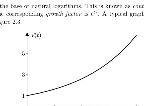
is the base of natural logarithms. This is known ascontinuous compounding. The corresponding growth factor is etr. A typical graph of V(t) is shown in
Figure 2.3.
Figure 2.3 Continuous compounding at 10% (r= 0.1,P = 1)
The derivative ofV(t) = etrP is
V′(t) =retrP =rV(t).
In the case of continuous compounding the rate of the growth is proportional to the current wealth.
2. Risk-Free Assets 33
Exercise 2.18
How long will it take to earn $1 in interest if $1,000,000 is deposited at 10% compounded continuously?
Exercise 2.19
In 1626 Peter Minuit, governor of the colony of New Netherland, bought the island of Manhattan from Indians paying with beads, cloth, and trinkets worth $24. Find the value of this sum in year 2000 at 5% com-pounded a) continuously and b) annually.
Proposition 2.2
Continuous compounding produces higher future value than periodic com-pounding with any frequencym, given the same initial principalP and interest rater.
Proof
It suffices to verify that
etr>(1 + r
m)
tm=(1 + r
m)
m r
rt .
The inequality holds because the sequence (1+r
m)
m
r is increasing and converges
to e asmր ∞.
Exercise 2.20
What will be the difference between the value after one year of $100 deposited at 10% compounded monthly and compounded continuously? How frequent should the periodic compounding be for the difference to be less than $0.01?
The present value under continuous compounding is obviously given by
V(0) =V(t)e−tr.
In this case the discount factor is e−tr. Given the terminal value V(T), we
clearly have
34 Mathematics for Finance
Exercise 2.21
Find the present value of $1,000,000 to be received after 20 years as-suming continuous compounding at 6%.
Exercise 2.22
Given that the future value of $950 subject to continuous compounding will be $1,000 after half a year, find the interest rate.
The returnK(s, t) defined by (2.3) on an investment subject to continuous compounding fails to be additive, just like in the case of periodic compounding. It proves convenient to introduce thelogarithmic return
k(s, t) = lnV(t)
V(s). (2.12)
Proposition 2.3
The logarithmic return is additive,
k(s, t) +k(t, u) =k(s, u).
Proof
This is an easy consequence of (2.12):
k(s, t) +k(t, u) = lnV(t)
V(s)+ ln
V(u)
V(t)
= lnV(t)
V(s)
V(u)
V(t) = ln
V(u)
V(s) =k(s, u).
IfV(t) is given by (2.10), thenk(s, t) =r(t−s), which enables us to recover the interest rate
r= k(s, t)
t−s .
Exercise 2.23
2. Risk-Free Assets 35
2.1.5 How to Compare Compounding Methods
As we have already noticed, frequent compounding will produce a higher fu-ture value than less frequent compounding if the interest rates and the initial principal are the same. We shall consider the general circumstances in which one compounding method will produce either the same or higher future value than another method, given the same initial principal.
Example 2.5
Suppose that certificates promising to pay $120 after one year can be purchased or sold now, or at any time during this year, for $100. This is consistent with a constant interest rate of 20% under annual compounding. If an investor decided to sell such a certificate half a year after the purchase, what price would it fetch? Suppose it is $110, a frequent first guess based on halving the annual profit of $20. However, this turns out to be too high a price, leading to the following arbitrage strategy:
• Borrow $1,000 to buy 10 certificates for $100 each.
• After six months sell the 10 certificates for $110 each and buy 11 new certificates for $100 each. The balance of these transactions is nil.
• After another six months sell the 11 certificates for $110 each, cashing $1,210 in total, and pay $1,200 to clear the loan with interest. The balance of $10 would be the arbitrage profit.
A similar argument shows that the certificate price after six months cannot be too low, say, $109.
The price of a certificate after six months is related to the interest rate under semi-annual compounding: If this rate isr,then the price is 1001 +r
2
dollars and vice versa. Arbitrage will disappear if the corresponding growth factor 1 + r
2
2
over one year is equal to the growth factor 1.2 under annual compounding,
36 Mathematics for Finance
Definition 2.1
We say that two compounding methods are equivalent if the corresponding growth factors over a period of one year are the same. If one of the growth factors exceeds the other, then the corresponding compounding method is said to bepreferable.
Example 2.6
Semi-annual compounding at 10% is equivalent to annual compounding at 10.25%. Indeed, in the former case the growth factor over a period of one year is
1 + 0.1 2
2
= 1.1025,
which is the same as the growth factor in the latter case. Both are preferable to monthly compounding at 9%, for which the growth factor over one year is only
1 +0.09 12
12
∼
= 1.0938.
We can freely switch from one compounding method to another equivalent method by recalculating the interest rate. In the chapters to follow we shall normally use either annual or continuous compounding.
Exercise 2.24
Find the rate for continuous compounding equivalent to monthly com-pounding at 12%.
Exercise 2.25
Find the frequency of periodic compounding at 20% to be equivalent to annual compounding at 21%.
Instead of comparing the growth factors, it is often convenient to compare the so-called effective rates as defined below.
Definition 2.2
For a given compounding method with interest rate r the effective rate re is