THE FLORIDA STATE UNIVERSITY
COLLEGE OF ARTS AND SCIENCES
FIRST MEASUREMENT OF TOP QUARK PAIR PRODUCTION CROSS-SECTION IN MUON PLUS HADRONIC TAU FINAL STATES
By
SUHARYO SUMOWIDAGDO
A Dissertation submitted to the Department of Physics in partial fulfillment of the requirements for the degree of
Doctor of Philosophy
The members of the Committee approve the Dissertation of Suharyo Sumowidagdo defended
on November 26, 2007.
Todd Adams
Professor Directing Dissertation
Ettore Aldrovandi
Outside Committee Member
Horst Wahl
Committee Member
Laura Reina
Committee Member
Simon Capstick Committee Member
A K U
Kalau sampai waktuku
’Ku mau tak seorang ’kan merayu Tidak juga kau
Tak perlu sedu sedan itu
Aku ini binatang jalang Dari kumpulannya terbuang
Biar peluru menembus kulitku Aku tetap meradang menerjang
Luka dan bisa kubawa berlari Berlari
Hingga hilang pedih perih
Dan aku akan lebih tidak perduli
Aku mau hidup seribu tahun lagi
Chairil Anwar, 1922-1949
So! now ’tis ended, like an old wife’s story
ACKNOWLEDGEMENTS
This dissertation could not have seen the light of the day without the hard work, dedication, and
support of many people. First of all, I thank members of the DØ Collaboration and the technical
staff of Fermilab that have provided world-class research facilities with their endless hard work,
days and nights.
I thank my advisor Todd Adams for being a patient advisor and sharing many wisdoms he has
about doing physics analysis. For allowing me to propose and carry out research on a topic of my
own, and keep supporting and working with me from the beginning until the end despite all the
difficulties and challenges faced.
To Harrison Prosper who has been a second advisor with many discussions I had with him, and
for his insights in shaping the analysis strategy. To Horst Wahl, Laura Reina, Simon Capstick, and
Ettore Aldrovandi for the time they spent serving in my graduate committee. Horst and Simon
provided many useful critics and suggestions which improve the manuscript. To the other faculty
members of the experimental high energy physics group at Florida State University, for all the
support you gave me all these years.
To members of the DØ Top Group who helped me one way or another during the time I was
working on the analysis. Amnon Harel and Dag Gilberg helped me getting started with the analysis
framework, and answered a lot of questions I raised. Amnon also helped when I worked on data
sets and Monte Carlo samples used in this analysis. Lisa Shabalina for her comments on the
analysis note, and her assistance with the evaluation of systematic uncertainties and cross-section
combination. Michele Weber for the data quality and luminosity calculation. Michael Begel for
many discussions I had with him, and for repeatedly putting me back on track.
To members of the DØ Tau Identification Group for developing and establishing tau
identifica-tion algorithm. To members of my editorial board for the time they spent on reviewing the analysis
version of the dissertation.
To the Florida State University people at Fermilab: Andrew, Bill, Dan, Daekwang, Edgar,
Jadranka, Jose, Norm, Oleksiy, Silke, and Trang. Thanks for the time we spent together, and
putting up with my antics at the office. For Andrew, Dan, and Oleksiy: thank you for your
cheerful attitudes which helped me relieving a lot of tension off my head. Silke Nelson taught me a
lot about tau identification algorithm during the earlier phase of this analysis. Daekwang Kau and
I joined DØ together in the summer of 2002, and he has been a good friend since then. Especially
during the tough period we had together during dissertation writing and defense phase.
To Kathy Mork of the High Energy Physics Office; Sherry Tointigh of the Graduate Student
Office; Joy Ira, Marjorie Fontalvo and Erin Skelly of the International Student Center. Thank you
for helping me through all the bureaucracy and paperwork related to travel, academic matters, and
immigration while I was away at Fermilab.
Down in the control room and deep inside the DØ Assembly Building, I had a demanding
but rewarding experience in working with Fritz Bartlett, Geoff Savage, Vladimir Sirotenko, Stan
Krzywdzinski, Dean Schamberger, Bill Lee, and Norm Buchanan. I have learned a lot from their
work ethics and attitudes. I will always remember that without hard work on the detector side,
there will never be any results on the physics side.
To my undergraduate professors at the Nuclear and Particle Theory Group, University of
Indonesia. Terry Mart introduced me to the real world of physics research, supervised my first
scientific work, and helped me to start a career in physics. The late Darmadi Kusno introduced
me to high-energy physics, taught me a lot of physics in and out of class, and always convinced me
that there is a real chance, despite all the hardships in Indonesia, to pursue a real career in physics.
May his soul rest in peace.
To my housemates Dan and Marco, for being a constant source of fun and entertaiment, and
for putting up with my rants and complains.
To my family who have always supported me ever since I decided to pursue a career in physics.
For allowing me to be far away in space and time. For always remembering me even during the
times when I forget about them and am swamped in my work. I can never thank them enough.
To Jutri Taruna and Alvin Kiswandhi, my sister and brother here in the United States, a place
so far away from our home country. It has been a long journey we’ve been through together. From
our days in Depok and Salemba. I couldn’t have done it without you, and words will never be
TABLE OF CONTENTS
List of Tables . . . ix
List of Figures . . . x
Abstract . . . xi
1. FOUNDATIONS . . . 1
1.1 The Standard Model of Particle Physics . . . 1
1.2 Top Quarks Production and Decay . . . 3
1.3 The Tau Lepton . . . 6
1.4 Research Motivations and Objectives . . . 7
1.4.1 Historical overview. . . 7
1.4.2 The importance of top decays to tau lepton. . . 8
1.5 Overview of the analysis’ approach . . . 8
1.6 Convention . . . 10
2. EXPERIMENTAL APPARATUS . . . 12
2.1 The Tevatron Accelerator . . . 12
2.2 The DØ Detector . . . 13
2.3 Central Tracking Detector . . . 14
2.4 Calorimeter and Inter-Cryostat Detector . . . 17
2.5 Muon Spectrometer . . . 19
2.6 Luminosity Monitor and Measurement . . . 21
2.7 Trigger and Data Acquisition System . . . 22
3. EVENT RECONSTRUCTION AND OBJECT IDENTIFICATION . . . . 26
3.1 Charged Particle Track Reconstruction . . . 26
3.2 Primary Vertex Reconstruction . . . 27
3.3 Muon Reconstruction . . . 28
3.4 Calorimeter Energy Clusters . . . 30
3.4.1 Simple cone algorithm . . . 30
3.4.2 Nearest-neighbor (CellNN) algorithm . . . 32
3.5 Reconstruction of Electromagnetic Objects . . . 33
3.6 Jet Reconstruction . . . 36
3.6.1 Jet energy corrections . . . 36
3.6.2 Identification ofb−quark jets . . . 39
4. TAU RECONSTRUCTION AND IDENTIFICATION . . . 44
4.1 Reconstruction of Tau Candidates . . . 45
4.2 Separation of Taus and Hadronic Jets using Neural Network . . . 47
5. EVENT PRESELECTION . . . 55
5.1 Data Set . . . 55
5.1.1 Trigger . . . 55
5.1.2 Data quality . . . 56
5.2 Monte Carlo Samples . . . 57
5.2.1 Monte Carlo generator and samples . . . 57
5.2.2 Heavy flavorK-factor . . . 57
5.2.3 Trigger efficiency corrections in Monte Carlo . . . 58
5.3 Preselection of Muon+Jets Events . . . 58
5.3.1 General strategy . . . 59
5.3.2 Muon+jets selection criteria . . . 59
5.3.3 Normalization ofW+jets events . . . 60
5.4 Selection of Tau Candidates in Muon+Jets Events . . . 61
5.4.1 Monte Carlo to data correction factor for jets faking taus . . . 66
5.5 Background Yield Estimation . . . 67
5.5.1 Multijet events . . . 67
5.5.2 Z+jets events . . . 69
5.5.3 Diboson events . . . 71
5.6 Analysis of Pre-tagged Sample . . . 71
6. MEASUREMENT OF σ(pp¯→t¯t) AND σ(pp¯→t¯t)·BR tt¯→µτhb¯b . . . 76
6.1 Estimation oft¯t Event Efficiency . . . 76
6.2 Analysis ofb−tagged Sample . . . 76
6.3 Cross-section Extraction . . . 79
6.4 Measurement ofσ(pp¯→tt¯)·BR(t¯t→µτhb¯b) . . . 81
6.5 Systematic Uncertainties . . . 82
6.6 Combinations with the electron+tau channel . . . 84
6.7 Conclusions and Outlook . . . 85
APPENDIX . . . 89
A. CONTROL PLOTS . . . 89
A.1 One-jet exclusive sample . . . 89
A.2 Two-jet inclusive sample . . . 93
REFERENCES . . . 101
LIST OF TABLES
1.1 The branching ratio ofW boson with adjustment to the observed final state objects.. 11
1.2 Branching ratios for varioust¯tfinal states, adjusted to the observed final state objects. 11
3.1 Input variables to the neural-network-based algorithm to identifyb−quark jets. . . 40 4.1 Basic properties of the three charged leptons. . . 44
4.2 Branching ratios (in unit of %) for dominant leptonic and hadronic decay modes of tau, sorted by expected tau type, as stated in [21]. . . 45
4.3 List of tau neural net input variables, and their usage by a particular tau type as input to their respective neural networks. . . 50
5.1 Names of datasets used in this analysis, and the number of events in each dataset. . 55
5.2 Trigger names and their respective luminosities in each trigger version range. . . 56
5.3 Summary of muon+jets selection criteria with some parameters and their effects on the muon+jets skim. . . 60
5.4 Number of events in data and Monte Carlo W+jets enriched sample. The Monte Carlo sample is normalized to the generator cross-section. . . 67
5.5 Observed/expected same-sign events in data at the pre-tagged level, and the expected amount of W+jets and t¯t lepton+jets events to be subtracted from SS data to get the estimation of multijet background contributions in the opposite sign (OS) sample. 69
5.6 Sum of ALPGEN LO cross-section across different parton-level multiplicity bins
for different mass ranges, the corresponding NLO theoretical cross-sections, and the relative scale factor between the two. Here the Z boson is decayed into one lepton flavor only. . . 69
5.7 List of Pythia diboson MC used in this analysis. . . 71
6.1 Efficiency of muon+tau+jets selection cuts on t¯t → dilepton and t¯t → µτhb¯b generated byALPGEN Monte Carlo. . . 77
6.2 Efficiency of muon+tau+jets selection cuts on tt¯→lepton+jets signal generated by
ALPGENMonte Carlo. . . . 78
6.3 Efficiencies of the muon+tau+jets selection fort¯tdilepton andtt¯lepton+jets sample, and the total efficiencies fort¯t→ inclusive sample. . . 78 6.4 Observed same-sign (SS) events in data at the tagged level, and the expected number
ofW+jets andtt¯lepton+jets events to be subtracted from SS data to get estimation of multijet background in the opposite sign (OS) sample. Notice the large statistical error on the SS data sample due to small statistics. . . 79
6.5 Estimated and observed yield for various component in the OS sample with at least two jets and at least oneb−tagged jet requirement. . . 80 6.6 Efficiencies of the muon+tau+jets selection with same-sign muon-tau pair for t¯t
dilepton andt¯tlepton+jets sample, and the total efficiencies fort¯t→inclusive sample. 81 6.7 Summary of statistical uncertainties on each of the sources of events in the µτ
channel. The SM cross section is used for t¯tproduction. . . 82
LIST OF FIGURES
1.1 Plots of electroweak constraints of the mass of the standar model Higgs particle from other standard model measurement. Top left: constraints from the mass of
W bosons, mW; top right: constraints from the mass of the top quark, mt; bottom left: constraints from both mass of the top quark and theW bosons, bottom right: constraints from the global electroweak fit. Figures are taken from the report of LEP Electroweak Working Group [1]. . . 2
1.2 Four leading-order Feynman diagrams for top quark pair production at the Tevatron. Upper figure is thes–channel quark fusion process. Lower figures, starting from left, are thes–channel,t–channel, andu–channel gluon fusion processes, respectively. . . 4
1.3 Feynman diagrams for leptonic and hadronic decay mode of top quark. . . 4
1.4 Summary of DØ measurements oft¯tcross-section at the Tevatron in various channels as of Winter 2007 [7]. . . 5
1.5 Illustrations for tau leptonic decay (left), tau hadronic one-prong decay (middle), and tau hadronic three-prong decay (right). Here h is a charged hadrons (mostly charged pions), and neutrals are either neutral pions or photons. . . 7
1.6 The strategy adapted by this analysis. . . 10
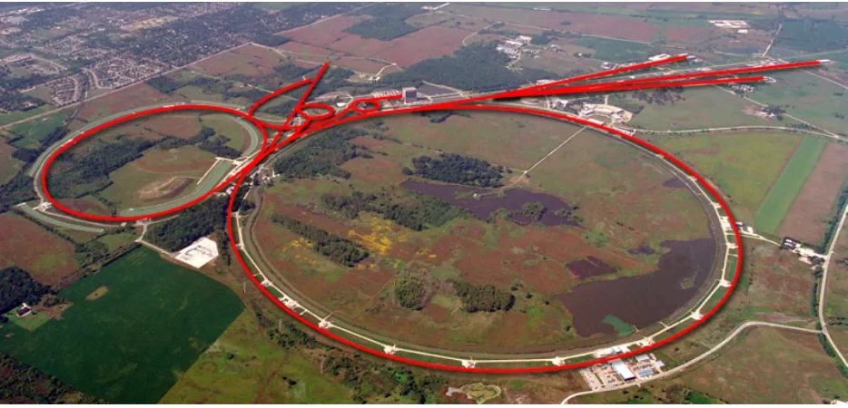
2.1 An aerial view of Fermilab, looking in the northwestward direction. The red lines show the schematic of the accelerator complex. Tevatron is the largest circle in the foreground. DØ detector is located at the building complex near the lower-right corner. 13
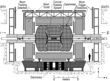
2.2 A side view of the DØ detector as seen from the West side of the detector. . . 14
2.3 The central tracking region of the DØ detector. . . 15
2.4 The DØ silicon microstrip tracker detector. . . 16
2.5 A complete φ segment of the forward preshower detector with the four layer of wedge-shaped detectors. . . 17
2.7 A schematic view of a calorimeter readout cell with its liquid argon gap and signal board. . . 19
2.8 Exploded view of the muon drift chambers. . . 20
2.9 Exploded view of the muon scintillators. . . 21
2.10 Schematic drawing of the luminosity detector and its location within the DØ detector. . . 22
2.11 Schematic display of data flow in DØ trigger and data acquisition system. . . 23
2.12 Flow diagrams of DØ Level 1 and Level 2 trigger systems, with the arrow lines show the flow of trigger information between subsystems. . . 25
3.1 Hollow cone used in defining muon calorimeter isolation variable. . . 29
3.2 Muon reconstruction correction factor as a function of muon detector η and φ. . . . 30
3.3 Muon track reconstruction correction factor as a function of CFT detector η, for different range of the track z−position. . . 31 3.4 Muon isolation correction factor as a function of muon detector η, for different
isolation criteria. The isolation criterion used in this analysis is TopScaledMedium. 32
3.5 Two different neighboring schemes in nearest-neighbor cell clustering algorithm. . . . 33
3.6 Merging of two seed cells in the 4-neighbors scheme and 8-neighbor scheme to one single merged cluster. . . 34
3.7 Evolution of a parton coming from hard scattering process into jet in the calorimeter. 37
3.8 Offset energy correction for different primary vertex multiplicities as a function of the jet detector pseudorapidity. . . 38
3.9 Schematic illustration of MPF method. . . 39
3.10 Relative response correction in data as a function of jet detector pseudorapidity. . . 40
3.11 Absolute response correction in data after offset and relative response corrections as a function of partially-corrected jet energy. . . 41
3.12 Showering correction in data as a function of corrected jet transverse energy. . . 42
3.13 Fractional jet energy scale uncertainties as a function of uncorrected jet transverse energy, plotted for three different pseudorapidity values. . . 43
4.2 Distributions of the N Nτ input variables for tau type 1. Black histogram is data, blue histogram is Monte CarloZ → τ τ, and red histogram is Monte CarloW → µ. All histograms are normalized to unit area. . . 51
4.3 Distributions of the N Nτ input variables for tau type 2. Black histogram is data, blue histogram is Monte CarloZ → τ τ, and red histogram is Monte CarloW → µ. All histograms are normalized to unit area. . . 52
4.4 Distributions of the N Nτ input variables for tau type 3. Black histogram is data, blue histogram is Monte CarloZ → τ τ, and red histogram is Monte CarloW → µ. All histogram is normalized to unit area. . . 53
4.5 Distributions of the tau NN output for all three types. The left column is a linear scale while the right is the same distribution with a logarithmic scale. The top row shows type 1 taus, the middle row is type 2 taus, while the bottom row is type 3 taus. The black histogram is data, the blue histogram is Z →τ τ MC (signal), and the red histogram isW →ℓν MC (fake tau). The histograms are normalized to unit area. . . 54
5.1 Distributions of the transverse mass from the muon+jets sample used to determine the W normalization factor. The filled histograms show the templates used in the fit and have been normalized using the results. Contributions from Z and tt¯have been subtracted from the data. . . 62
5.2 Distributions of control variables from the muon+jets sample including all contribu-tions (part 1 of 2). . . 63
5.3 Distributions of control variables from the muon+jets sample including all contribu-tions (part 2 of 2). . . 64
5.4 Distributions of tau neural net output (N Nτ) in the preselected muon+tau+jets sample before N Nτ cut. Left figure is for all values of N Nτ in logarithmic scale, right figure is for values ofN Nτ greater than 0.5 in linear scale. . . 65
5.5 Distributions of tau neural net output (N Nτ) in the preselected muon+tau+jets sample before N Nτ cut. Left figure is for all values of N Nτ in logarithmic scale, right figure is for values ofN Nτ greater than 0.5 in linear scale. . . 66
5.6 Distributions of the W transverse mass for the muon+jets sample. The top row shows the distributions where a muon and at least one jet are required. The bottom rows shows distributions where a tau is required to be found. The left are data (with
Z, multijet and t¯tsubtracted) while the right areW MC. . . 68
5.8 Distributions of control variables from normalization of Z/γ → µ−µ+ by invariant
mass template fit. . . 73
5.9 Distributions of control variables in the preselected muon+tau+jets sample (Part 1 of 2) . . . 74
5.10 Distributions of control variables in the preselected muon+tau+jets sample (Part 2 of 2) . . . 75
6.1 Plots of some distributions in the sample with at least two jets one of which isb-tagged. 86
ABSTRACT
This dissertation presents the first measurement of top quark pair production cross-section in
events containing a muon and a tau lepton. The measurement was done with 1 fb−1 of data
collected during April 2002 through February 2006 using the DØ detector at the Tevatron
proton-antiproton collider, located at Fermi National Accelerator Laboratory (Fermilab), Batavia, Illinois.
Events containing one isolated muon, one tau which decays hadronically, missing transverse energy,
and two or more jets (at least one of which must be tagged as a heavy flavor jet) were selected.
Twenty-nine candidate events were observed with an expected background of 9.16 events. The top
quark pair production cross-section is measured to be
σ(t¯t) = 8.0+2−2..48 (stat)+1−1..87(syst)±0.5 (lumi) pb.
Assuming a top quark pair production cross-section of 6.77 pb for Monte Carlo signal top events
without a real tau, the measuredσ×BR is
CHAPTER 1
FOUNDATIONS
1.1
The Standard Model of Particle Physics
This dissertation presents an investigation in the field of elementary particle physics, whose goal
is to understand the fundamental constituents of matters and the laws governing them. The
standard model (SM) is the currently accepted theory which describes a vast range of phenomena
in elementary particle physics, including the strong, weak, and electromagnetic interactions. It is
consistent, renormalizable, and has been tested in precision to a high degree of accuracy.
There are two key features of the standard model. The first one is gauge invariance, which means
the physics described by the standard model should not change under phase transformations which
are functions of space-time coordinates. The second is the Higgs mechanism, the formalism which
endows the particles of the standard model with mass.
The gauge invariance principle constrains the particle contents and the interactions between
them in a unique way. Given a set of particles, the symmetry group of transformation, and the
gauge bosons, the principle defines the form of interactions between the particles mediated by the
bosons. The standard model is a theory based on theSU(3)C×SU(2)L×U(1)Y symmetry groups. The subscript C, L, and Y refers to the color group, left-handed, weak isospin group, and weak
hypercharge group, respectively.
A theory of fundamental particle interactions built from the gauge invariance principle alone
doesn’t allow the existence of massive gauge bosons. In the standard model, the masses of the
gauge bosons of weak interactions are generated by the Higgs mechanism. It transforms degrees
of freedom in the Higgs field(s), which are scalar field(s), into masses of the weak gauge bosons.
In elementary particle theory, the Higgs mechanism that generates these masses is also known
as electroweak symmetry breaking. Within the electroweak theory, the Higgs mechanism is also
80.3 80.4 80.5
10 102 103
mH [GeV]
mW
[
GeV
]
Excluded
High Q2 except mW/ΓW
68% CL
mW (LEP2 prel., pp − )
160 180 200
10 102 103
mH [GeV]
mt
[
GeV
]
Excluded
High Q2 except mt 68% CL
mt (Tevatron)
80.3 80.4 80.5
150 175 200
mH [GeV]
114 300 1000
mt [GeV]
mW
[
GeV
]
68% CL
∆α LEP1 and SLD
LEP2 and Tevatron (prel.)
0 1 2 3 4 5 6
100
30 300
mH [GeV]
∆χ
2
Excluded Preliminary
∆αhad = ∆α(5)
0.02758±0.00035 0.02749±0.00012
incl. low Q2 data
Theory uncertainty
mLimit = 144 GeV
There is no unique formulation of the Higgs mechanism in the standard model. It is therefore
more custom to use the termHiggs sector when discussing the more general aspects of electroweak
symmetry breaking and the origin of mass of standard model fermion. In the standard model, the
minimal implementation of the Higgs mechanism is an SU(2) doublet which corresponds to the
existence of an electrically neutral, scalar particle.
A tremendous amount of effort has been put to explore and understand the Higgs sector of the
standard model. As of the year 2007, there is no direct experimental confirmation of the physics
of the Higgs sector, be it the minimal one or any of the extended ones. The available knowledge
about the Higgs sector is obtained by constraints from other parts of the standard model. Figure
1.1 shows four graphs that show the constraints on the minimal standard model Higgs from other
well-measured parameters of the standard model.
An important property of the Higgs particles1 is that the couplings between Higgs particles
and other particles are proportional to the other particles’ masses. The top quark is currently the
heaviest known particle, and is expected to play important role in the exploration of electroweak
symmetry breaking mechanism. The next section discusses top quark production and decays at
the Tevatron.
1.2
Top Quarks Production and Decay
In 1995, two major collaborations at Fermilab announced the discovery of the top quark [2, 3].
It was observed in the form of t¯t or top quark-antiquark pair production (hereby will be loosely
addressed by the term “top quark pair”). The discovery verified the previous theoretical prediction
for the existence of three generations of quarks. Due to the small amount of data, enormous
backgrounds, and tight cuts in triggering and analysis, each of the collaborations could obtain only
tens of top quark events. Those events were just enough for both groups to claim observation. Using
the complete data set recorded from 1992 to 1996 at the Tevatron2, the collaborations were able
to measure the top quark mass and top quark pair production cross section at the corresponding
center-of-mass energy.
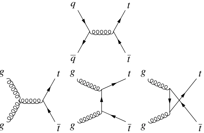
Figure 1.2 shows the four leading-order Feynman diagrams for top quark pair production at the
Tevatron via strong interaction. At the Tevatron’s center-of-momentum (c.m.) energy of 1.96 TeV,
the quark fusion process dominates (85%) over the gluon fusion (15%) processes in contributing
1Plural form is chosen.
q
q
t
t
g
g
t
t
g
g
t
t
g
g
t
t
Figure 1.2: Four leading-order Feynman diagrams for top quark pair production at the Tevatron. Upper figure is the s–channel quark fusion process. Lower figures, starting from left, are the s– channel,t–channel, andu–channel gluon fusion processes, respectively.
W
t
b
ℓ
ν
ℓ
W
t
b
q
′
q
Figure 1.3: Feynman diagrams for leptonic and hadronic decay mode of top quark.
toward the total cross-section. The theoretical prediction at next-to-leading order for pp¯ → t¯t
cross-section at√s= 1.96 TeV is about 6.8±0.8 pb [4, 5]. DØ’s most precise measurement of the
t¯tcross-section is
σpp¯→t¯t= 8.3−+00..65 (stat) −+01..90 (syst) ±0.5 (lumi) pb.
as reported in Ref. [6].
Figure 1.4: Summary of DØ measurements of tt¯cross-section at the Tevatron in various channels as of Winter 2007 [7].
displayed in Figure 1.3. Any other decay modes (if they exist) have not been observed. In the case
of tt¯production, the decays of the two W bosons determine the final state. The W bosons can
decay into either a charged lepton-neutrino pair (eνe,µνµ, andτ ντ), or quark-anti quark pair. The
branching ratio (neglecting decay kinematics and CKM suppression) is 19 for each lepton flavor,
and 13 for each qq′ mode. Thus, for the case oft¯tone has
1. equal dilepton channel, where both W bosons decay to the same lepton flavor (ee,µµ, τ τ),
2. unequal dilepton channel, where the twoW bosons decay to different lepton flavors (eµ, eτ,
µτ), each channel with BR of 812.
3. lepton+jets channels, where one W boson decays into a lepton-neutrino pair, and the other
W boson decays to a quark-antiquark pair (e+ jets, µ + jets, and τ + jets), each channel
with BR of 274.
4. all jets channel where bothW bosons decay intoqq′ final states, with BR 4 9.
Measurement of t¯t cross-section has been performed by DØ in several dilepton channels (ee,
µµ, eµ) [8, 9], lepton+jets channels (e+jets, µ+jets, τ+jets) [10–13], and the all hadronic channel
[14]. Figure 1.4 shows a comparison of DØ results ont¯tcross-section measurements in the different
channels as of Winter 2007. All measurements are done with the assumptions of top massmt= 175
GeV and standard model decay of top quarks. It can be seen that most of the experimental effort
to study top quark events have been focusing on channels involving electrons, muons, and jets only.
The tau sector in top decay has lagged behind the other channels.
1.3
The Tau Lepton
The tau lepton was discovered in 1975 at the Stanford Linear Accelerator Center [15]. Physicists
from the MARK I Collaboration observed events in e+e− collisions whose final states have two
leptons with different flavor
e+e−→e±µ∓+ 2 or more undetected particles.
The explanation for those events is production of a new lepton pair,τ+τ−, which later decays into
e/µand neutrinos.
The tau has properties similar to the two lighter leptons, electron and muon, except for mass,
and lifetime. Its mass is 1.77 GeV/c2, heavier even than a proton, roughly an order of magnitude
heavier than the muon, and three orders of magnitude heavier than the electron. Conservation
of lepton number means that tau can only decays through charged-current weak interaction via
emission of a virtual W boson. It can decays into leptonic final states (eνeντ and µνµντ) or
hadronic final states (charged and neutral mesons). The lifetime of the tau lepton is extremely
short, 2.9×10⁻¹³ seconds, withcτ = 87µm.
This analysis will focus on the hadronic decay modes of tau leptons. Figure 1.5 shows
W
τ
ν
τ
ν
e
,
ν
µ
e
,
µ
τ
ν
τ≥
0
π
0/
K
0h
±(
π
±,
K
±)
τ
ν
τ≥
0
π
0/
K
0h
±¡
π
±,
K
±¢
h±
¡
π
±,
K
±¢
h
±¡
π
±,
K
±¢
Figure 1.5: Illustrations for tau leptonic decay (left), tau hadronic one-prong decay (middle), and tau hadronic three-prong decay (right). Here h is a charged hadrons (mostly charged pions), and neutrals are either neutral pions or photons.
The decay modes into one charged hadron are also known as “one-prong” decays, while the decay
modes into three charged hadrons are known as “three-prong” decays. The hadrons in tau decay
are strongly dominated by pions. In more than 60% cases of all hadronic decays, one or more
neutral pion which decays into two photons appear(s) in the final states. In almost all cases, tau
hadronic decays will appear as narrow jets, sometimes accompanied with electromagnetic showers.
1.4
Research Motivations and Objectives
Analyses of dilepton modes of top quark production/decay benefit from relatively small backgrounds
but suffer from small branching ratios. By including hadronic taus explicitly in t¯t analyses, two
goals are achieved at once. The first goal is improvement of t¯t dilepton analyses by the addition
of a final state which was not feasible before. This analysis will improve the statistics for dilepton
analyses by adding one of the remaining three channels. The combination of this channel and
the electron+tau channel is one of the larger dilepton samples. The second goal is to extend the
sensitivity oft¯tanalysis to include aspects to which muon or electron identification is not sensitive,
but tau identification is.
1.4.1 Historical overview.
Prior to this work, all searches for top quark decays into the muon/electron+hadronic tau decay
channel have been done by CDF. The first used approximately 110 pb−1 of Run I data [16]. A
second search involved about 200 pb−1 Run II data [17]. Finally, two searches were done using
production [19].
In Run II, DØ performed an analysis using approximately 350 pb−1 of data to measure the top
quark production cross-section in theτ + jets channel [13]. The measured value is
σpp¯→t¯t= 5.1−+43..35 (stat)−+00..77(syst)±0.3(lumi) pb.
This value is the first DØ result using top quark decay to a tau lepton. This work presented here
will complement theτ+jets results by including theµ+τ channel.
1.4.2 The importance of top decays to tau lepton.
The decay of top quarks into tau lepton,t→ τ ντb is a pure third generation decay. As such, this
decay is a unique probe to new physics, which alters the top quark decay modes into states that
favor subsequent decay to taus rather than other standard model particles.
A well-known candidate for new physics in t → τ X decay is the existence of charged Higgs
boson, with mass mH < mt−mb [20]. If such a particle exists, the top quark could decay into
a charged Higgs plus a b quark (t → Hb) in addition to the known W boson plus b quark. The
charged Higgs is expected to decay preferentially into a tau, which is the heaviest lepton.
t→H±b→τ ντb (1.1)
In some theories beyond the minimal Higgs sector of the standard model, the top quark decay to
H±b is even more favored than the SM decay into W b. A precise measurement of top quark pair
production cross section in decay channels involving hadronic taus will provide a way to test such
theories.
1.5
Overview of the analysis’ approach
From the viewpoint of the physical processes that contribute to the final states, this analysis has
the characteristics of t¯tdilepton analyses such as:
1. Small branching ratio fromt¯tinitial state.
2. The presence of two leptons with opposite-sign charges.
3. The presence of large missing transverse energy which is strongly correlated with the two
However, hadronic taus have a similar signature to jets, and can be faked by jets. Therefore, this
analysis also has the characteristics of a t¯tmuon+jets analysis. This dual feature oftt¯muon+tau
analysis is crucial in forming the analysis strategy. Many aspects of the analysis from triggering,
the choices of data sets, background composition and estimation, have been strongly influenced by
t¯tdilepton and muon+jets analyses.
There are two primary categories of backgrounds to be considered. The first type comprises
events with a real isolated muon and a real isolated hadronic tau. The primary source of this
background is the Drell-Yan processZ/γ∗ →τ−τ++ jets with final states in which one of the taus
decays to a muon, and the other tau decays hadronically. Since tau decays produce one or more
neutrinos, Drell-YanZ/γ∗ →τ τ + jets will have real missing transverse energy. Other significant
SM processes with a similar signature are the diboson (W W, W Z, and ZZ) events in which the
bosons decay into two or more leptons with taus included.
The second background category has an object which is misidentified as an isolated hadronic
tau. This misidentified object can be an electron, a muon, or a jet. There are two primary sources
of this type of background. The first source is the processZ/γ∗ →µ−µ++ jets. The second source
involves a jet falsely reconstructed as a tau lepton. Multijet events and production of W bosons
with jets are examples. While the efficiency of jets to pass the tau identification algorithm is small,
the large cross-sections make this background non-negligible.
This analysis selects events with one isolated high-pT muon, one isolated hadronic tau, large
missing transverse energy, and two high-pT jets. Because this leaves large multijet, W and Z/DY
backgrounds, this analysis appliesb−tagging to take advantage of the heavy quark content of the
top decays relative to the much smaller heavy quark content of the background.
After applying b−tagging, the sample is dominated by top quark events. These events are a
mixture ofµ+τh + 2ν + 2b, other dilepton andµ/e+ jets events, whereτh is a tau lepton which
decays hadronically. A two staged analysis is performed.
1. First, the top production cross-section is measured using all available top events. This result
can be combined with other measurements by accounting for any overlap between samples.
2. Second, the cross-section×branching ratio for the specific final states,t¯t→µ+τh+ 2ν+ 2b,
is measured as a step toward tests of universality and searches for a charged Higgs boson.
Figure 1.6 shows a flow diagram of the analysis strategy. We select a muon+jets sample that
Selection of muon+jets events
↓
Normalization of W+jets background
↓
Selection of tau in muon+jets events
ւց
Opposite charge sign muon+tau pair
↓
Cross-section measurement
Same charge sign muon+tau pair
↓
Multijet background estimation
Figure 1.6: The strategy adapted by this analysis.
of the major background. The, we proceed to select a tau in the muon+jets sample, effectively
selecting a muon+tau+jets sample. We then divide the muon+tau+jets sample into two disjoint
samples. The first sample contains lepton-tau pairs with opposite charge sign (OS). This sample
contains the signal events, and the cross-section measurement will be done using this sample. The
second sample contains the muon-tau pairs with same-sign charge (SS). This sample will be used
to estimate multijet background in the OS sample.
1.6
Convention
Throughout this document, the following terms are used:
τh: Aτ lepton which decays to hadron(s) and a tau neutrino.
τe: A τ lepton which decays to an electron, an electron neutrino, and a tau neutrino.
τµ: A τ lepton which decays to a muon, a muon neutrino, and a tau neutrino.
To aid in understanding of how this analysis is different from, and how it is related to, the
other t¯tanalyses, the meaning of a particular t¯t final state is redefined in terms ofthe set of final
objects which are actually seen by the detector. For example, the decay W →τ ντ →e(µ)νe(µ)ντ is
assigned to the observable final statee(µ). Table 1.1 lists theW branching ratio after combination
of the decayW →e(µ)νeµ with the decay W →τ ντ → e(µ)νe(µ)ντ, where the values of W and τ
branching ratios have been taken from the 2006 Particle Data Book [21].
With the observed final states of W boson decays as given in Table 1.1, one can compute the
branching ratio into observed final states of tt¯decays, with the assumption that the top quark
Table 1.1: The branching ratio ofW boson with adjustment to the observed final state objects..
ObservableW decay Branching ratio
BR (e) = BR (W →eνe) + BR (W →τ ντ →eνeντντ) 0.1276 BR (µ) = BR (W →µνµ) + BR (W →τ ντ →µνµντντ) 0.1252 BR (τh) = BR (W →τ ντ)×BR (τ →hadrons +ντ) 0.0729
BR (qq′) 0.6743
Table 1.2: Branching ratios for various t¯tfinal states, adjusted to the observed final state objects.
Decay modes Value
BR (t¯t→ee) BR (e)×BR (e) 0.01628 BR (t¯t→eµ) 2×BR (e)×BR (µ) 0.03195 BR (t¯t→eτh) 2×BR (e)×BR (τh) 0.01860 BR (t¯t→µµ) BR (µ)×BR (µ) 0.01568 BR (t¯t→µτh) 2×BR (µ)×BR (τh) 0.01825 BR (t¯t→τhτh) BR (τh)×BR (τh) 0.00531
BR (t¯t→ℓℓ),(ℓ∈ {e, µ, τ}) BR (ℓ)×BR (ℓ) 0.10608
BR (t¯t→e+ jets) 2×BR (e)×BR (qq′) 0.17208 BR (t¯t→µ+ jets) 2×BR (µ)×BR (qq′) 0.16884 BR (t¯t→τh+ jets) 2×BR (τh)×BR (qq′) 0.09831 BR (t¯t→ℓ+ jets),(ℓ∈ {e, µ, τ}) 2×BR (ℓ)×BR (qq′) 0.43924 BR (t¯t→alljets) BR (qq′)×BR (qq′) 0.45468
CHAPTER 2
EXPERIMENTAL APPARATUS
The work presented in this dissertation was done utilizing two major experimental facilities in high
energy physics. The first is the Tevatron accelerator which provides beams of high energy particles.
The second is the DØ detector which provides a means to study results of collision of high energy
particle beams from the Tevatron. Both are located at Fermi National Accelerator Laboratory in
Batavia, Illinois.
2.1
The Tevatron Accelerator
The Tevatron is a storage ring that collides high-energy proton and antiproton beams. Each beam
has an energy of 980 TeV, making the total center-of-momentum (c.m.) energy in the collision
processes to be 1.96 TeV. Tevatron has a diameter of approximately 2 km. Figure 2.1 shows an
aerial picture of the Tevatron and other accelerators at Fermilab. Viewed from above, the proton
beam circulates in the clockwise direction, while antiproton beam circulates in the counter-clockwise
direction. There are six designated points on the Tevatron where the beams are made to cross with
each other. At two of those six points, named B0 and D0, the beams are made to collide with each other. The DØ detector is located at theD0collision point, hence the origin of the name.
The Tevatron operates by circulating bunches of particles instead of continuous beams. There
are 36 bunches each of protons and antiprotons. At the two mentioned collision points, crossings of
protons and antiprotons bunches happen every 396 ns. Typical values of instantaneous luminosity
(L) delivered by the Tevatron are 1031−1032 cm−2 sec−1.
The amount of data recorded by the DØ detector is expressed in units of luminosity integrated
over time (cm−2). A convenient way to express this unit is to convert it into another unit which
has the dimension of inverse area. Commonly accepted units are pb−1 (1036 cm−2 ) or fb−1
Figure 2.1: An aerial view of Fermilab, looking in the northwestward direction. The red lines show the schematic of the accelerator complex. Tevatron is the largest circle in the foreground. DØ detector is located at the building complex near the lower-right corner.
2.2
The DØ Detector
The DØ detector is a general purpose particle detector designed to study hard scattering processes in
proton-antiproton collisions at the TeV energy scale. The detector has three principal subsystems:
central tracking detectors, a hermetic uranium/liquid argon calorimeter, and muon spectrometer.
Figure 2.2 shows a side view of the detector. An exhaustive description of the DØ detector is
available [22].
A right-handed coordinate system is used to describe the detector and physics events. The
z−axis is directed along the direction of the proton beam, and the y−axis is directed upward.
The polar angle θ is the angle between a vector from the origin and the positive z−axis. In
addition, it is convenient to define the two quantities pseudorapidity and transverse momentum.
The pseudorapidity is defined as:
η =−ln
tan
θ
2
(2.1)
which approximates the true rapidityy,
η = 1
2ln
E+pzc
E−pzc
Figure 2.2: A side view of the DØ detector as seen from the West side of the detector.
in the massless approximation, (mc2/E) → 0. The region which has a large value of |η| is called
“forward”. The transverse momentum (pT) is defined as the component of momentum projected
onto a plane perpendicular to the beam axis.
pT =psinθ (2.3)
Two choices of the coordinate system’s origin are used: the reconstructed primary vertex of pp¯
interaction and the center of the detector. The first one is referred as the physics coordinate, and
the second one is referred as detector coordinate.
2.3
Central Tracking Detector
The central tracking detector consists of the silicon microstrip tracker (SMT), the central fiber
Figure 2.3: The central tracking region of the DØ detector.
tracking system of DØ detector. The SMT and CFT are located within a cylindrical volume inside
the magnet with approximate length of 2.5 m and radius of 50 cm. The solenoidal magnet generates
a nearly uniform magnetic field along thez−direction with a strength of 2 T. Together, the central
tracking detectors allow reconstruction of charged particle tracks and independent measurement
of their momenta, precise determination of the primary vertex, and reconstruction of secondary
vertices to identify heavy quark jets.
The SMT consists of silicon detectors in the form of barrel modules and disk modules. Figure
2.4 shows a three-dimensional rendering of the SMT detector. There are six barrel modules, each
Figure 2.4: The DØ silicon microstrip tracker detector.
along the beam direction. Two larger disks are located further in the z−direction to cover the
forward region. The barrel detectors provide positional measurement in the transverse plane, while
the disk detectors provide measurement in the longitudinal direction as well as in the transverse
plane. The radius of the smaller disk modules in the middle part is 10 cm, while the larger disk at
the ends have a radius of 26 cm.
The CFT consists of sixteen layers of scintillating fibers which are mounted on eight cylindrical
support structures. The innermost cylinder has a radius of approximately 20 cm while the
outermost radius has a radius of approximately 50 cm. Each cylinder supports two doublet layers
of scintillating fibers: one with the fibers oriented parallel with the beam (z), and one with the
fibers oriented at a stereo angle of either +3◦ (u) or−3◦ (v). Starting from the innermost cylinder,
the layers are arranged in the sequence: zu−zv−zu−zv−zu−zv−zu−zv−zu−zv. The
scintillating fibers are connected optically to clear fiber waveguides which send the optical signal
further to the readout electronics.
The solenoidal magnet provides almost uniform magnetic field of strength 2 T along the
z−direction. The TOSCA [23] program is used to model the magnetic field map within the detector.
A study withJ/ψ→ µ+µ− events shows that the the magnetic field map is accurate within 0.5%
precision. The magnet operates at a temperature of 10 K and draws a current of approximately
4750 A.
The preshower detector has a role of both calorimeter and tracking detectors. It aids in the
identification of electrons, photons, and pions from tau decays. The preshower detector is divided
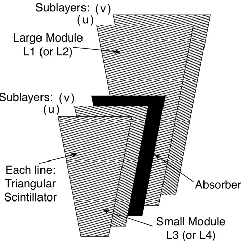
Figure 2.5: A completeφsegment of the forward preshower detector with the four layer of wedge-shaped detectors.
the forward preshowers detectors (FPS) which cover the region 1.5<|η|<2.5.
The CPS is located between the solenoidal magnet and the central calorimeter module. It
consists of three concentric, cylindrical layers of scintillating fibers. One layer has axial orientation,
and two layers have stereo orientation of approximately±24◦. The FPS are attached to the faces of
the endcap calorimeter modules. They have the form of disks built from wedge-shaped segments.
Each segment has two layers of scintillating fibers with different orientation, separated by an angle
of 22.5◦. Figure 2.5 shows a complete segment of the FPS detector.
2.4
Calorimeter and Inter-Cryostat Detector
The DØ calorimeter system is built from three uranium/liquid-argon, sampling calorimeters and
inter-cryostat detector (ICD). The central calorimeter (CC) covers the region of detector|η|<1.0,
and the two endcap calorimeters (EC) cover the region 1.4<|η|<4.2. The calorimeters operate at
a temperature of 90 K and each of them is contained within its own cryostat. Between the central
and the endcap calorimeters are the ICD detectors which are built from scintillating tile detectors.
They provide readout in the region where the calorimeters have incomplete coverage.
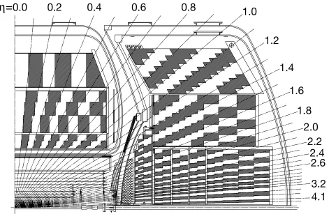
Figure 2.6: A side view of a quarter of the calorimeter, showing the segmentation of the calorimeter into cells and towers. The rays from the center of the detector are rays of contanst pseudorapidity.
in η−φ space. Figure 2.6 shows a side view of a quarter of the calorimeter, together with the
rays which show the projective towers. In the radial outward direction, each tower is divided into
cells which are grouped further into different type of layers. From inside to outside, the layers
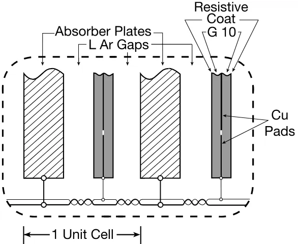
are: electromagnetic, fine hadronic, and coarse hadronic. Figure 2.7 shows a schematic view of a
calorimeter cell.
Each type of layer uses a different design of absorber plate for its readout cells. The
electromagnetic layers use thin plates (3-mm-thick in CC or 4-mm-thick in EC) made of nearly
depleted uranium. The fine hadronic layers use 6-mm-thick plates made of uranium-niobium alloy
in both CC and EC. The coarse hadronic layers use 46.5-mm-thick copper plates (in EC) or stainless
Figure 2.7: A schematic view of a calorimeter readout cell with its liquid argon gap and signal board.
layers have a much higher noise level compared to the electromagnetic and fine hadronic layers.
The electromagnetic layers play an important role in the reconstruction of electrons, photons,
and taus. There are four layers of electromagnetic readout modules both in CC and EC. The EM
layers cover the region up to|η|<2.5, with a gap in the interval 1.1<|η|<1.5, which corresponds
to the region between CC and EC. Of particular importance is the third EM layer which has
spatial resolution of 0.05×0.05, twice that of the other layers . This finer resolution aids in precise
reconstruction of electrons, photons, and neutral pions from tau decays.
2.5
Muon Spectrometer
The muon spectrometer is divided into the central muon detector and two forward muon detectors.
The central muon detector covers the region up to|η|<1.0, while the forward muon detectors cover
the region in the range 1.0<|η|<2.0. There are two main components used to build the detectors:
drift chambers and scintillation counters. The drift chambers provide spatial information, while
the scintillation counters provide fast and precise timing measurement for triggering and positional
measurement.
Figure 2.8: Exploded view of the muon drift chambers.
and a toroidal magnet. There are three layers of drift chambers, one is located within the magnet
(A layer), and two outside (B and C layer). Two layers of scintillation counters are installed, one
right inside the A layer and one right outside the C layer.
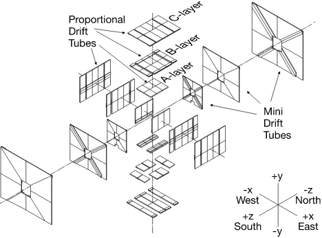
The forward muon detectors consist of mini drift tubes (MDT) and scintillation counters. They
are arranged in three layers, each layer has both MDTs and scintillators. Similar to the central
muon detectors, there is one layer inside the toroidal magnet and two layers outside the toroidal
magnets.
Figure 2.8 and Figure 2.9 show the expanded views of the muon chambers and muon scintillators,
Figure 2.9: Exploded view of the muon scintillators.
2.6
Luminosity Monitor and Measurement
The luminosity detector is built of two arrays of 24 wedge-shaped scintillation counters and
photomultiplier tube (PMT) attached into each wedge. They are located at the front of the endcap
calorimeters, covering the pseudorapidity region 2.7 < |η|< 4.4, as can be seen in Figure 2.3. A
zoomed drawing, focusing on the luminosity monitor only, can be found in Figure 2.10.
The instantaneous luminosity of pp¯ collisions in the DØ detector’s interaction region is
determined by measuring the counting rate of inelasticpp¯collisions,
L= 1
σeff
dN
dt (2.4)
whereL is the instantaneous luminosity, σeff is the effective inelasticpp¯cross-section (taking into
Figure 2.10: Schematic drawing of the luminosity detector and its location within the DØ detector.
rate measured by the detector. To eliminate background from beam halo, the origin of collisions
must be within|z|<100.0 cm. The origin of collisions is estimated from the time of flights recorded
at the two sides of the luminosity counter.
In practice, the counting rate is determined by counting the fraction of beam crossing with
no collisions recorded, and then use Poison statistics to determine dNdt . This method is known as
thecounting zeros technique, and it ensures that multiple collisions are treated properly [24]. The
measurement is done over a time period which is short enough to ensure that the instantaneous
luminosity is constant throughout the period, and long enough to make the statistical uncertainty
on the counting rate negligible. This time period is known as luminosity block. A unique number
(luminosity block number) is assigned to each luminosity block. The calculation of total integrated
luminosity for a given data is done by integrating the instantaneous luminosity over time, treating
each luminosity block as a timeslice in the integration.
2.7
Trigger and Data Acquisition System
The DØ detector uses a three-level trigger system to reduce the number of readout events to
approximately 50-100 Hz for recording to tape. Figure 2.11 shows an overview of the triggering
and data acquisition system.
The first level (Level 1 or L1) takes input from the central tracking detector, calorimeter, and
Figure 2.11: Schematic display of data flow in DØ trigger and data acquisition system.
such as:
• Hit patterns in the central tracking detector consistent with a charged particle above a certain
pT threshold.
• Energy depositions in the calorimeter above a certain energy threshold, either on the electromagnetic layers only, or on the full tower.
• Hits in the muon chambers and muon scintillators above a minimum number of hits.
Candidate events passing the L1 requirement are then sent to the the next level (Level 2 or L2).
The Level 2 trigger consists of subdetector-specific processing nodes, and a global node which
tests for correlation between information across the subdetectors. The detector-specific nodes
can perform simple reconstruction of physics objects using information only from their assigned
subdetector. The L2 trigger is designed to have a maximum accept rate of 850 Hz.
Figure 2.12 shows the flow of information from various sub-detectors into the L1 and L2 trigger
system.
The last level, Level 3 (L3), consists of two subsystems: The Level 3 Data Acquisition Cluster
(L3 DAQ) and Level 3 filter. The L3 DAQ is an event builder which reads event information
from all subdetectors and reconstructs complete physics objects in the event. Simplified versions
of the reconstruction algorithms are used here as there is a time constraint during data taking.
event information. The L3 filter applies more complicated selection criteria such as requirements
of isolation, object-matching, or object-separation. The final output of the L3 trigger has a rate of
approximately 50-100 Hz.
Events which pass all three trigger levels are written temporarily onto local disks on the online
data-taking cluster. The data are later transferred into a robotic tape system for further
post-recording reconstruction and processing.
It is convenient to define three kind of events that are recorded by the DØ detector:
• Zero bias: events which are recorded without any requirements on the trigger. The content of those events is dominated by readout electronics’ noises and energy deposited by cosmic
muons.
• Minimum bias: events which are recorded with a requirement that a proton-antiproton collision has happened in the detector. In addition to the content of zero bias events, they
also contains energy coming from underlying events.
Level2
Detector Level1
Framework
Trigger
Lumi
L2
Global
L2MUO
L2STT
L2CTT
L2PS
L1CTT
L1MUO
L1FPD
FPD
MUO
SMT
CFT
CAL
L1CAL
CPS
FPS
L2CAL
CHAPTER 3
EVENT RECONSTRUCTION AND OBJECT
IDENTIFICATION
The reconstruction process which converts raw data from the DØ detector proceeds in three steps:
1. Conversion of raw data into hits which correspond to position and energy measurement.
2. Reconstruction of basic physics objects: charged particle tracks in the tracking detector,
clusters of energies in the calorimeters, and tracks in the muon system.
3. Combination of basic physics objects into final physics objects: electrons, photons, muons,
taus, jets, and vertices.
This chapter describes the principal ideas of reconstruction algorithms for physics objects at
DØ with the exception of taus, which require an in-depth treatment. Chapter 4 describes the
reconstruction of taus in detail.
3.1
Charged Particle Track Reconstruction
Reconstruction of charged particle tracks uses information exclusively from the central tracking
detectors. There are two steps in the reconstruction process: candidate track finding and track
fitting.
In the first step, two methods are used to build a list of candidate tracks. The first one uses
histograms to find patterns of particle trajectories among hit clusters in the tracking detector
[25]. It is based on a Hough transformation which was originally used to find patterns in bubble
chamber pictures [26]. The second one uses hit clusters in the SMT to form roads, onto which hits
in additional tracking detector layers are added [27].
In the second step, the list of candidate tracks from the first step are passed to a track fitter
DØ interacting propagator [30], which is a generic black box algorithm that propagates a track in
the DØ tracking system, taking into account the DØ solenoid’s magnetic field and interaction of
charged particles with detector material. For each candidate track, the algorithm incrementally
adds hit clusters associated with the candidate track into the fit and recalculates the optimal track
parameters. This step is repeated until all hit cluster information has been used.
3.2
Primary Vertex Reconstruction
The primary vertex is the origin of tracks from hard scattering processes in pp¯ collisions. The
algorithm’s goal is to separate the primary vertex from vertices produced in minimum-bias
interactions and decays of long-lived particles. There are three steps in the primary vertex
reconstruction algorithm: track clustering and selection, vertex fitting, and vertex selection [31].
In the first step, tracks are clustered along the z−direction. The clustering algorithm begins
with the track which has the highest pT and adds tracks to the cluster if the z−distance between
the track and the cluster is less than 2 cm. Tracks are required to havepT >0.5 GeV, at least two
(zero) SMT hits if they are inside (outside) the SMT geometrical acceptance region. At the end
of this step is a list of candidate vertices which may contain the hard scatter primary vertex and
additional vertices from minimum bias interactions and decay of long-lived particles.
In the second step, a two-pass algorithm is used for eachz−cluster to fit the clustered tracks to
a common vertex. In the first pass, a tear-down K´alm´an vertex fitter fits all tracks into a common
vertex, and removes the track which contributes the largestχ2 into the fit. The fit is repeated until
the totalχ2/n.d.o.f.of the fit is less than 10.
In the second pass, the tracks in eachz−cluster are first sorted in order of their distance of closest
approach (DCA) in the x−y plane to the beam spot, using beam-spot information determined
in the first pass. Only tracks which have significance (defined as |DCA|/σDCA) less than 5.0 are
selected. The selected tracks are then fitted to a common vertex with an adaptive K´alm´an vertex
fitter. The fitter weighs theχ2 contribution of each track by a Fermi function,
wi =
1 1 +e(χ2
i−χ2c)/2T
(3.1)
where χ2i is the χ2 contribution of the track to the vertex fit, χ2c is the cutoff value, and T is a
parameter which determines the sharpness of the function [31].
In the last step, a probabilistic method is used to determine the primary vertex. The method
distribution. The vertex which has the smallest probability to be a minimum bias vertex is selected
as the primary vertex [32].
3.3
Muon Reconstruction
Muons are identified by using hit information in the muon system and tracks reconstructed by the
central tracking detector [33]. The algorithm begins by combining scintillator and wire chamber
hits into trajectories in the muon system (called local muons) which are consistent with muons
coming from the interaction region. Reconstructed local muons are then matched with tracks in
the tracking detector. Here it is necessary to propagate tracks from the central tracking detector to
the muon system [34]. The final reconstructed, track-matched muons use the tracks’ information
to obtain the muons’ charge and momenta.
In this analysis, two definitions of muon are used, one is a subset of the other one.
• Loose muon
1. The muon is required to have wire and scintillator hits inside and outside the muon
toroid.
2. Muon is required to have scintillator hit times to be less than 10 ns from the time a
bunch crossing happens. This cut helps to to reject cosmic muons.
3. The muon must be matched to a track in the central tracking detector. The track is
required to have a good fit withχ2/n.d.o.f. <4.0 and the distance of closest approach
(|DCA|) to the primary vertex to be less than 0.2 cm for tracks without hits in the
silicon detector. For tracks which have hits in the silicon detector, the DCA requirement
is tightened to|DCA|<0.02 cm.
4. The muon is separated from jets which havepT at least 15.0 GeV by ∆R >0.5 in η−φ
space. This condition is called loose isolation condition.
• Tight muon
Tight muons are required to fulfill the loose muon requirements and the tight isolation
conditions. The conditions for a tight isolation are:
1. The sum of calorimeter transverse energy in an annular cone with inner radius 0.1 and
µ
R = 0.1
R = 0.4
Figure 3.1: Hollow cone used in defining muon calorimeter isolation variable.
momentum,
PcellsE
T
pµT
<0.15, (3.2)
The sum is performed over all calorimeter cells within the cone with the exception of
cells within the coarse hadronic layers. Figure 3.1 shows the definition of hollow cone
used in calculating the muon calorimeter isolation.
2. The momentum sum of all tracks (excluding the muon track) in a cone of radius 0.5 (in
η−φspace) around the muon direction, must be less than 15 % of the muon transverse
momentum.
Ptracks
pT
pµT
<0.15, (3.3)
In Monte Carlo events, the efficiency to reconstruct a muon is corrected to simulate the efficiency
in data. For each reconstructed muon in the event, a correction factor is multiplied to the event’s
weight. An exhaustive table of the correction factor as function of muon kinematics is determined
by using the tag-and-probe method in dimuon data sample and inZ →µ+µ−Monte Carlo sample.
The correction factor is broken down into correction for muon detector hits reconstruction, muon
track reconstruction, and muon isolation in the tracking detector and calorimeter.
Figure 3.2 to Figure 3.4 shows distributions of efficiency corrections factors for muon
reconstruc-tion, broken down into the three different corrections mentioned earlier. The average correction
values in top signal Monte Carlo for muon hit reconstruction, muon track reconstruction, and muon
η Muon detector
-2.5 -2 -1.5 -1 -0.5 0 0.5 1 1.5 2 2.5
φ
Muon detector
0 1 2 3 4 5 6
0 0.2 0.4 0.6 0.8 1 eff_eta_phi_muid_medium_nseg3
Figure 3.2: Muon reconstruction correction factor as a function of muon detectorη andφ.
3.4
Calorimeter Energy Clusters
Reconstruction of energy cluster in the calorimeter is a principal step in identification of electrons,
photons, taus, and jets. Two basic algorithms used to reconstruct calorimeter cluster will be
discussed: the simple cone algorithm and the nearest-neighbor cell algorithm.
3.4.1 Simple cone algorithm
The simple cone algorithm uses a list of towers to build clusters which become input to more specific
algorithms which reconstruct jets, electrons, photons and taus. The algorithm takes calorimeter
towers as input and proceeds in the following steps:
1. All towers above a certain threshold ire collected in a list L, which is sorted in order of
decreasing towerET.
CFT eta, z<-39 -2.5 -2 -1.5 -1 -0.5 0 0.5 1 1.5 2 2.5
ε
0 0.2 0.4 0.6 0.8 1
eff_cft_eta_track_medium_bin_0
CFT eta, -39<z<-10 -2.5 -2 -1.5 -1 -0.5 0 0.5 1 1.5 2 2.5
ε
0 0.2 0.4 0.6 0.8 1
eff_cft_eta_track_medium_bin_1
CFT eta, -10<z<10 -2.5 -2 -1.5 -1 -0.5 0 0.5 1 1.5 2 2.5
ε
0 0.2 0.4 0.6 0.8 1
eff_cft_eta_track_medium_bin_2
CFT eta, 10<z<39 -2.5 -2 -1.5 -1 -0.5 0 0.5 1 1.5 2 2.5
ε
0 0.2 0.4 0.6 0.8 1
eff_cft_eta_track_medium_bin_3
CFT eta, z>39 -2.5 -2 -1.5 -1 -0.5 0 0.5 1 1.5 2 2.5
ε
0 0.2 0.4 0.6 0.8 1
eff_cft_eta_track_medium_bin_4
Figure 3.3: Muon track reconstruction correction factor as a function of CFT detectorη, for different range of the trackz−position.
3. The algorithm then loops over the remaining towers in the list. If the algorithm finds a tower
J whose distance from the current clusterC, ∆R(C, J) is less than Rcone, whereRcone is the
radius parameter of the algorithm, then the towerJ is added to the clusterC and removed
from the list of towers.
4. When the algorithm has reached the end of the list of towers, then the current cluster is
added to the list of clusters.
5. Steps 1 to 4 are repeated until there are no more towers in the tower list.
The simple cone algorithm uses three key parameters: the minimum energy of a tower to be
considered in the list of towers, the minimum energy of a tower to be combined with the current

![Figure 1.4: Summary of DØ measurements of tt¯ cross-section at the Tevatron in various channelsas of Winter 2007 [7].](https://thumb-ap.123doks.com/thumbv2/123dok/3383830.1759512/20.612.157.494.74.464/figure-summary-measurements-section-tevatron-various-channelsas-winter.webp)