Information Theory and Network Coding pdf pdf

(1)

(2)

(3)

Raymond W. Yeung

Information Theory and

Network Coding

SPIN Springer’s internal project number, if known

May 31, 2008

(4)

(5)

(6)

(7)

Preface

This book is an evolution from my bookA First Course in Information Theory published in 2002 when network coding was still at its infancy. The last few years have witnessed the rapid development of network coding into a research field of its own in information science. With its root in information theory, network coding not only has brought about a paradigm shift in network com-munications at large, but also has had significant influence on such specific research fields as coding theory, networking, switching, wireless communica-tions, distributed data storage, cryptography, and optimization theory. While new applications of network coding keep emerging, the fundamental results that lay the foundation of the subject are more or less mature. One of the main goals of this book therefore is to present these results in a unifying and coherent manner.

While the previous book focused only on information theory for discrete random variables, the current book contains two new chapters on information theory for continuous random variables, namely the chapter on differential entropy and the chapter on continuous-valued channels. With these topics included, the book becomes more comprehensive and is more suitable to be used as a textbook for a course in an electrical engineering department.

What is in this book

Out of the twenty-one chapters in this book, the first sixteen chapters belong to Part I,Components of Information Theory, and the last five chapters belong to Part II, Fundamentals of Network Coding. Part I covers the basic topics in information theory and prepare the reader for the discussions in Part II. A brief rundown of the chapters will give a better idea of what is in this book.

(8)

Chapter 2 introduces Shannon’s information measures for discrete random variables and their basic properties. Useful identities and inequalities in in-formation theory are derived and explained. Extra care is taken in handling joint distributions with zero probability masses. There is a section devoted to the discussion of maximum entropy distributions. The chapter ends with a section on the entropy rate of a stationary information source.

Chapter 3 is an introduction to the theory ofI-Measure which establishes a one-to-one correspondence between Shannon’s information measures and set theory. A number of examples are given to show how the use of informa-tion diagrams can simplify the proofs of many results in informainforma-tion theory. Such diagrams are becoming standard tools for solving information theory problems.

Chapter 4 is a discussion of zero-error data compression by uniquely de-codable codes, with prefix codes as a special case. A proof of the entropy bound for prefix codes which involves neither the Kraft inequality nor the fundamental inequality is given. This proof facilitates the discussion of the redundancy of prefix codes.

Chapter 5 is a thorough treatment of weak typicality. The weak asymp-totic equipartition property and the source coding theorem are discussed. An explanation of the fact that a good data compression scheme produces almost i.i.d. bits is given. There is also an introductory discussion of the Shannon-McMillan-Breiman theorem. The concept of weak typicality will be further developed in Chapter 10 for continuous random variables.

Chapter 6 contains a detailed discussion of strong typicality which applies to random variables with finite alphabets. The results developed in this chap-ter will be used for proving the channel coding theorem and the rate-distortion theorem in the next two chapters.

The discussion in Chapter 7 of the discrete memoryless channel is an en-hancement of the discussion in the previous book. In particular, the new def-inition of the discrete memoryless channel enables rigorous formulation and analysis of coding schemes for such channels with or without feedback. The proof of the channel coding theorem uses a graphical model approach that helps explain the conditional independence of the random variables.

Chapter 8 is an introduction to rate-distortion theory. The version of the rate-distortion theorem here, proved by using strong typicality, is a stronger version of the original theorem obtained by Shannon.

In Chapter 9, the Blahut-Arimoto algorithms for computing the channel capacity and the rate-distortion function are discussed, and a simplified proof for convergence is given. Great care is taken in handling distributions with zero probability masses.

(9)

Preface IX

distributions echos the section in Chapter 2 on maximum entropy distribu-tions.

Chapter 11 discusses a variety of continuous-valued channels, with the continuous memoryless channel being the basic building block. In proving the capacity of the memoryless Gaussian channel, a careful justification is given for the existence of the differential entropy of the output random variable. Based on this result, the capacity of a system of parallel/correlated Gaus-sian channels is obtained. Heuristic arguments leading to the formula for the capacity of the bandlimited white/colored Gaussian channel are given. The chapter ends with a proof of the fact that zero-mean Gaussian noise is the worst additive noise.

Chapter 12 explores the structure of theI-Measure for Markov structures. Set-theoretic characterizations of full conditional independence and Markov random field are discussed. The treatment of Markov random field here maybe too specialized for the average reader, but the structure of theI-Measure and the simplicity of the information diagram for a Markov chain is best explained as a special case of a Markov random field.

Information inequalities are sometimes called the laws of information the-ory because they govern the impossibilities in information thethe-ory. In Chap-ter 13, the geometrical meaning of information inequalities and the relation between information inequalities and conditional independence are explained in depth. The framework for information inequalities discussed here is the basis of the next two chapters.

Chapter 14 explains how the problem of proving information inequalities can be formulated as a linear programming problem. This leads to a complete characterization of all information inequalities provable by conventional tech-niques. These inequalities, called Shannon-type inequalities, can be proved by the World Wide Web available software package ITIP. It is also shown how Shannon-type inequalities can be used to tackle the implication problem of conditional independence in probability theory.

Shannon-type inequalities are all the information inequalities known dur-ing the first half century of information theory. In the late 1990’s, a few new inequalities, called non-Shannon-type inequalities, were discovered. These in-equalities imply the existence of laws in information theory beyond those laid down by Shannon. In Chapter 15, we discuss these inequalities and their ap-plications.

(10)

Chapter 17 starts Part II of the book with a discussion of the butterfly network, the primary example in network coding. Variations of the butterfly network are analyzed in detail. The advantage of network coding over store-and-forward in wireless and satellite communications is explained through a simple example. We also explain why network coding with multiple infor-mation sources is substantially different from network coding with a single information source.

In Chapter 18, the fundamental bound for single-source network coding, called the max-flow bound, is explained in detail. The bound is established for a general class of network codes.

In Chapter 19, we discuss various classes of linear network codes on acyclic networks that achieve the max-flow bound to different extents. Static net-work codes, a special class of linear netnet-work codes that achieves the max-flow bound in the presence of channel failure, is also discussed. Polynomial-time algorithms for constructing these codes are presented.

In Chapter 20, we formulate and analyze convolutional network codes on cyclic networks. The existence of such codes that achieve the max-flow bound is proved.

Network coding theory is further developed in Chapter 21. The scenario when more than one information source are multicast in a point-to-point acyclic network is discussed. An implicit characterization of the achievable information rate region which involves the framework for information inequal-ities developed in Part I is proved.

How to use this book

1

2 3

4

10

17 Part II

Part I

18 19 20 21

5

6

7

12

13 14 15 16

8

(11)

Preface XI

Part I of this book by itself may be regarded as a comprehensive textbook in information theory. The main reason why the book is in the present form is because in my opinion, the discussion of network coding in Part II is in-complete without Part I. Nevertheless, except for Chapter 21 on multi-source network coding, Part II by itself may be used satisfactorily as a textbook on single-source network coding.

An elementary course on probability theory and an elementary course on linear algebra are prerequisites to Part I and Part II, respectively. For Chapter 11, some background knowledge on digital communication systems would be helpful, and for Chapter 20, some prior exposure to discrete-time linear systems is necessary. The reader is recommended to read the chapters according to the above chart. However, one will not have too much difficulty jumping around in the book because there should be sufficient references to the previous relevant sections.

This book inherits the writing style from the previous book, namely that all the derivations are from the first principle. The book contains a large number of examples, where important points are very often made. To facilitate the use of the book, there is a summary at the end of each chapter.

This book can be used as a textbook or a reference book. As a textbook, it is ideal for a two-semester course, with the first and second semesters cov-ering selected topics from Part I and Part II, respectively. A comprehensive instructor’s manual is available upon request. Please contact the author at whyeung@ie.cuhk.edu.hk for information and access.

Just like any other lengthy document, this book for sure contains errors and omissions. To alleviate the problem, an errata will be maintained at the book homepage http://www.ie.cuhk.edu.hk/IT book2/.

Hong Kong, China Raymond W. Yeung

(12)

(13)

Acknowledgments

The current book, an expansion of my previous book A First Course in In-formation Theory, is written within the year 2007. Thanks to the generous support of the Friedrich Wilhelm Bessel Research Award from the Alexan-der von Humboldt Foundation of Germany, I had the luxury of working on the project full-time from January to April when I visited Munich University of Technology. I would like to thank Joachim Hagenauer and Ralf Koetter for nominating me for the award and for hosting my visit. I also would like to thank Department of Information Engineering, The Chinese University of Hong Kong, for making this arrangement possible.

There are many individuals who have directly or indirectly contributed to this book. First, I am indebted to Toby Berger who taught me information theory and writing. I am most thankful to Zhen Zhang, Ning Cai, and Bob Li for their friendship and inspiration. Without the results obtained through our collaboration, the book cannot possibly be in its current form. I would also like to thank Venkat Anantharam, Vijay Bhargava, Dick Blahut, Agnes and Vin-cent Chan, Tom Cover, Imre Csisz´ar, Tony Ephremides, Bob Gallager, Bruce Hajek, Te Sun Han, Jim Massey, Prakash Narayan, Alon Orlitsky, Shlomo Shamai, Sergio Verd´u, Victor Wei, Frans Willems, and Jack Wolf for their support and encouragement throughout the years. I also would like to thank all the collaborators of my work for their contribution and all the anonymous reviewers for their useful comments.

(14)

(15)

1 The Science of Information

In a communication system, we try to convey information from one point to another, very often in a noisy environment. Consider the following scenario. A secretary needs to send facsimiles regularly and she wants to convey as much information as possible on each page. She has a choice of the font size, which means that more characters can be squeezed onto a page if a smaller font size is used. In principle, she can squeeze as many characters as desired on a page by using a small enough font size. However, there are two factors in the system which may cause errors. First, the fax machine has a finite resolution. Second, the characters transmitted may be received incorrectly due to noise in the telephone line. Therefore, if the font size is too small, the characters may not be recognizable on the facsimile. On the other hand, although some characters on the facsimile may not be recognizable, the recipient can still figure out the words from the context provided that the number of such characters is not excessive. In other words, it is not necessary to choose a font size such that all the characters on the facsimile are recognizable almost surely. Then we are motivated to ask: What is the maximum amount of meaningful information which can be conveyed on one page of facsimile?

This question may not have a definite answer because it is not very well posed. In particular, we do not have a precise measure of meaningful informa-tion. Nevertheless, this question is an illustration of the kind of fundamental questions we can ask about a communication system.

(22)

difficult to devise a measure which can quantify the amount of information contained in a piece of music.

In 1948, Bell Telephone Laboratories scientist Claude E. Shannon (1916-2001) published a paper entitled “The Mathematical Theory of Communi-cation” [322] which laid the foundation of an important field now known as information theory. In his paper, the model of a point-to-point communication system depicted in Figure 1.1 is considered. In this model, a message is

gener-TRANSMITTER

SIGNAL RECEIVED SIGNAL

MESSAGE MESSAGE

NOISE SOURCE INFORMATION

SOURCE RECEIVER DESTINATION

Fig. 1.1.Schematic diagram for a general point-to-point communication system.

ated by the information source. The message is converted by the transmitter into a signal which is suitable for transmission. In the course of transmission, the signal may be contaminated by a noise source, so that the received signal may be different from the transmitted signal. Based on the received signal, the receiver then makes an estimate on the message and deliver it to the destination.

In this abstract model of a point-to-point communication system, one is only concerned about whether the message generated by the source can be delivered correctly to the receiver without worrying about how the message is actually used by the receiver. In a way, Shannon’s model does not cover all possible aspects of a communication system. However, in order to develop a precise and useful theory of information, the scope of the theory has to be restricted.

(23)

1 The Science of Information 3

and the remaining task is to deliver these bits to the receiver correctly with no reference to their actual meaning. This is the foundation of all modern digital communication systems. In fact, this work of Shannon appears to contain the first published use of the term “bit,” which stands forbinary digit.

In the same work, Shannon also proved two important theorems. The first theorem, called the source coding theorem, introduces entropy as the funda-mental measure of information which characterizes the minimum rate of a source code representing an information source essentially free of error. The source coding theorem is the theoretical basis for losslessdata compression1_.

The second theorem, called thechannel coding theorem, concerns communica-tion through a noisy channel. It was shown that associated with every noisy channel is a parameter, called the capacity, which is strictly positive except for very special channels, such that information can be communicated reliably through the channel as long as the information rate is less than the capacity. These two theorems, which give fundamental limits in point-to-point commu-nication, are the two most important results in information theory.

In science, we study the laws of Nature which must be obeyed by any phys-ical systems. These laws are used by engineers to design systems to achieve specific goals. Therefore, science is the foundation of engineering. Without science, engineering can only be done by trial and error.

In information theory, we study the fundamental limits in communica-tion regardless of the technologies involved in the actual implementacommunica-tion of the communication systems. These fundamental limits are not only used as guidelines by communication engineers, but they also give insights into what optimal coding schemes are like. Information theory is therefore the science of information.

Since Shannon published his original paper in 1948, information theory has been developed into a major research field in both communication theory and applied probability.

For a non-technical introduction to information theory, we refer the reader toEncyclopedia Britannica[49]. In fact, we strongly recommend the reader to first read this excellent introduction before starting this book. For biographies of Claude Shannon, a legend of the 20th Century who had made fundamental contribution to the Information Age, we refer the readers to [56] and [340]. The latter is also a complete collection of Shannon’s papers.

Unlike most branches of applied mathematics in which physical systems are studied, abstract systems of communication are studied in information theory. In reading this book, it is not unusual for a beginner to be able to understand all the steps in a proof but has no idea what the proof is leading to. The best way to learn information theory is to study the materials first and come back at a later time. Many results in information theory are rather subtle, to the extent that an expert in the subject may from time to time realize that his/her

1 _{A data compression scheme is lossless if the data can be recovered with an}

(24)

(25)

Part I

(26)

(27)

2 Information Measures

Shannon’s information measuresrefer to entropy, conditional entropy, mutual information, and conditional mutual information. They are the most impor-tant measures of information in information theory. In this chapter, we in-troduce these measures and establish some basic properties they possess. The physical meanings of these measures will be discussed in depth in subsequent chapters. We then introduce the informational divergence which measures the “distance” between two probability distributions and prove some useful inequalities in information theory. The chapter ends with a section on the entropy rate of a stationary information source.

2.1 Independence and Markov Chains

We begin our discussion in this chapter by reviewing two basic concepts in probability: independence of random variables and Markov chain. All the ran-dom variables in this book except for Chapters 10 and 11 are assumed to be discrete unless otherwise specified.

LetX be a random variable taking values in an alphabetX. The probabil-ity distribution forXis denoted as{pX(x), x∈ X }, withpX(x) = Pr{X=x}.

When there is no ambiguity, pX(x) will be abbreviated as p(x), and {p(x)}

will be abbreviated as p(x). The supportof X, denoted by SX, is the set of

all x_{∈ X} such that p(x) >0. If _SX =X, we say thatp is strictly positive.

Otherwise, we say thatpis not strictly positive, orpcontains zero probability masses. All the above notations naturally extend to two or more random vari-ables. As we will see, probability distributions with zero probability masses are very delicate, and they need to be handled with great care.

Definition 2.1.Two random variablesX andY are independent, denoted by

X _⊥Y, if

p(x, y) =p(x)p(y) (2.1)

(28)

For more than two random variables, we distinguish between two types of independence.

Definition 2.2 (Mutual Independence). For n _≥ 3, random variables

X1, X2,· · ·, Xn are mutually independent if

p(x1, x2,· · ·, xn) =p(x1)p(x2)· · ·p(xn) (2.2)

for allx1, x2,· · ·,xn.

Definition 2.3 (Pairwise Independence). For n _≥ 3, random variables

X1, X2,· · ·, Xnare pairwise independent ifXi andXj are independent for all

1_≤i < j_≤n.

Note that mutual independence implies pairwise independence. We leave it as an exercise for the reader to show that the converse is not true.

Definition 2.4 (Conditional Independence).For random variablesX, Y, andZ,X is independent of Z conditioning on Y, denoted byX ⊥Z|Y, if

p(x, y, z)p(y) =p(x, y)p(y, z) (2.3)

for allx, y, andz, or equivalently,

p(x, y, z) =

(

p(x,y)p(y,z)

p(y) =p(x, y)p(z|y)if p(y)>0

0 otherwise. (2.4)

The first definition of conditional independence above is sometimes more convenient to use because it is not necessary to distinguish between the cases

p(y) > 0 andp(y) = 0. However, the physical meaning of conditional inde-pendence is more explicit in the second definition.

Proposition 2.5.For random variables X, Y, and Z, X ⊥Z|Y if and only if

p(x, y, z) =a(x, y)b(y, z) (2.5)

for allx,y, andz such thatp(y)>0.

Proof. The ‘only if’ part follows immediately from the definition of conditional independence in (2.4), so we will only prove the ‘if’ part. Assume

p(x, y, z) =a(x, y)b(y, z) (2.6)

for allx,y, and zsuch thatp(y)>0. Then for suchx,y, andz, we have

p(x, y) =X

z

p(x, y, z) =X

z

a(x, y)b(y, z) =a(x, y)X

z

(29)

(30)

Proof. This follows directly from the symmetry in the definition of a Markov chain in (2.15). ⊓⊔

In the following, we state two basic properties of a Markov chain. The proofs are left as an exercise.

Proposition 2.8.X1→X2 → · · · →Xn forms a Markov chain if and only

if

X1→X2→X3

(X1, X2)→X3→X4

.. .

(X1, X2,· · ·, Xn−2)→Xn−1→Xn

(2.17)

form Markov chains.

Proposition 2.9.X1→X2 → · · · →Xn forms a Markov chain if and only

if

p(x1, x2,· · ·, xn) =f1(x1, x2)f2(x2, x3)· · ·fn−1(xn−1, xn) (2.18)

for allx1, x2,· · ·,xn such thatp(x2), p(x3),· · ·, p(xn−1)>0.

Note that Proposition 2.9 is a generalization of Proposition 2.5. From Proposition 2.9, one can prove the following important property of a Markov chain. Again, the details are left as an exercise.

Proposition 2.10 (Markov subchains). Let _Nn = {1,2,· · ·, n} and let

X1→X2→ · · · →Xn form a Markov chain. For any subsetαofNn, denote

(Xi, i ∈α) by Xα. Then for any disjoint subsets α1, α2,· · ·, αm of Nn such

that

k1< k2<· · ·< km (2.19)

for allkj ∈αj,j= 1,2,· · ·, m,

Xα1→Xα2→ · · · →Xαm (2.20)

forms a Markov chain. That is, a subchain of X1→X2 → · · · →Xn is also

a Markov chain.

Example 2.11.Let X1 → X2 → · · · → X10 form a Markov chain and

α1 ={1,2}, α2 ={4}, α3 ={6,8}, andα4={10} be subsets of N10. Then

Proposition 2.10 says that

(X1, X2)→X4→(X6, X8)→X10 (2.21)

(31)

2.1 Independence and Markov Chains 11

We have been very careful in handling probability distributions with zero probability masses. In the rest of the section, we show that such distributions are very delicate in general. We first prove the following property of a strictly positive probability distribution involving four random variables1_.

Proposition 2.12.Let X1, X2, X3, and X4 be random variables such that

p(x1, x2, x3, x4) is strictly positive. Then

X1⊥X4|(X2, X3)

X1⊥X3|(X2, X4)

⇒X1⊥(X3, X4)|X2. (2.22)

Proof. IfX1⊥X4|(X2, X3), then

p(x1, x2, x3, x4) =

p(x1, x2, x3)p(x2, x3, x4)

p(x2, x3)

. (2.23)

On the other hand, ifX1⊥X3|(X2, X4), then

p(x1, x2, x3, x4) =

p(x1, x2, x4)p(x2, x3, x4)

p(x2, x4)

. (2.24)

Equating (2.23) and (2.24), we have

p(x1, x2, x3) = p(x2, x3)p(x1, x2, x4)

p(x2, x4)

. (2.25)

Therefore,

p(x1, x2) =

X

x3

p(x1, x2, x3) (2.26)

=X

x3

p(x2, x3)p(x1, x2, x4)

p(x2, x4)

(2.27)

= p(x2)p(x1, x2, x4)

p(x2, x4)

, (2.28)

or

p(x1, x2, x4)

p(x2, x4)

= p(x1, x2)

p(x2)

. (2.29)

Hence from (2.24),

p(x1, x2, x3, x4) =

p(x1, x2, x4)p(x2, x3, x4)

p(x2, x4) =

p(x1, x2)p(x2, x3, x4)

p(x2) (2.30)

for allx1, x2, x3, andx4, i.e., X1⊥(X3, X4)|X2. ⊓⊔

(32)

If p(x1, x2, x3, x4) = 0 for some x1, x2, x3, and x4, i.e., p is not strictly

positive, the arguments in the above proof are not valid. In fact, the propo-sition may not hold in this case. For instance, let X1 = Y, X2 = Z, and

X3=X4= (Y, Z), whereY and Z are independent random variables. Then

X1 ⊥ X4|(X2, X3), X1 ⊥ X3|(X2, X4), but X1 6⊥ (X3, X4)|X2. Note that

for this construction, pis not strictly positive because p(x1, x2, x3, x4) = 0 if

x36= (x1, x2) orx46= (x1, x2).

The above example is somewhat counter-intuitive because it appears that Proposition 2.12 should hold for all probability distributions via a continuity argument2 _{which would go like this. For any distribution} _p_{, let}

{pk} be a

sequence of strictly positive distributions such that pk → pand pk satisfies

(2.23) and (2.24) for allk, i.e.,

pk(x1, x2, x3, x4)pk(x2, x3) =pk(x1, x2, x3)pk(x2, x3, x4) (2.31)

and

pk(x1, x2, x3, x4)pk(x2, x4) =pk(x1, x2, x4)pk(x2, x3, x4). (2.32)

Then by the proposition,pk also satisfies (2.30), i.e.,

pk(x1, x2, x3, x4)pk(x2) =pk(x1, x2)pk(x2, x3, x4). (2.33)

Lettingk_{→ ∞}, we have

p(x1, x2, x3, x4)p(x2) =p(x1, x2)p(x2, x3, x4) (2.34)

for all x1, x2, x3, and x4, i.e., X1 ⊥ (X3, X4)|X2. Such an argument would

be valid if there always exists a sequence {pk} as prescribed. However, the

existence of the distribution p(x1, x2, x3, x4) constructed immediately after

Proposition 2.12 simply says that it is not always possible to find such a sequence{pk}.

Therefore, probability distributions which are not strictly positive can be very delicate. For strictly positive distributions, we see from Proposition 2.5 that their conditional independence structures are closely related to the fac-torization problem of such distributions, which has been investigated by Chan [60].

2.2 Shannon’s Information Measures

We begin this section by introducing the entropy of a random variable. As we will see shortly, all Shannon’s information measures can be expressed as linear combinations of entropies.

(33)

2.2 Shannon’s Information Measures 13 Definition 2.13.The entropyH(X) of a random variableX is defined as

H(X) =₋X

x

p(x) logp(x). (2.35)

In the definitions of all information measures, we adopt the convention that summation is taken over the corresponding support. Such a convention is necessary becausep(x) logp(x) in (2.35) is undefined ifp(x) = 0.

The base of the logarithm in (2.35) can be chosen to be any convenient real number greater than 1. We write H(X) asHα(X) when the base of the

logarithm is α. When the base of the logarithm is 2, the unit for entropy is thebit. When the base of the logarithm ise, the unit for entropy is thenat. When the base of the logarithm is an integer D ≥2, the unit for entropy is the D-it (D-ary digit). In the context of source coding, the base is usually taken to be the size of the code alphabet. This will be discussed in Chapter 4. In computer science, a bit means an entity which can take the value 0 or 1. In information theory, the entropy of a random variable is measured in bits. The reader should distinguish these two meanings of a bit from each other carefully.

Let g(X) be any function of a random variable X. We will denote the expectation ofg(X) byEg(X), i.e.,

Eg(X) =X

x

p(x)g(x), (2.36)

where the summation is over SX. Then the definition of the entropy of a

random variableX can be written as

H(X) =₋Elogp(X). (2.37)

Expressions of Shannon’s information measures in terms of expectations will be useful in subsequent discussions.

The entropy H(X) of a random variable X is a functional of the prob-ability distribution p(x) which measures the average amount of information contained in X, or equivalently, the average amount of uncertaintyremoved upon revealing the outcome ofX. Note thatH(X) depends only onp(x), not on the actual values in_X. Occasionally, we also denoteH(X) byH(p).

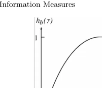
For 0_≤γ_≤1, define

hb(γ) =−γlogγ−(1−γ) log(1−γ) (2.38)

with the convention 0 log 0 = 0, so thathb(0) =hb(1) = 0. With this

conven-tion,hb(γ) is continuous at γ= 0 and γ= 1.hb is called thebinary entropy

function. For a binary random variableX with distribution{γ,1−γ},

H(X) =hb(γ). (2.39)

Figure 2.1 is the plot ofhb(γ) versusγin the base 2. Note thathb(γ) achieves

(34)

γ

Fig. 2.1.hb(γ) versusγin the base 2.

The definition of thejoint entropy of two random variables is similar to the definition of the entropy of a single random variable. Extension of this definition to more than two random variables is straightforward.

Definition 2.14.The joint entropy H(X, Y) of a pair of random variables

X andY is defined as

H(X, Y) =₋X

x,y

p(x, y) logp(x, y) =₋Elogp(X, Y). (2.40)

For two random variables, we define in the following theconditional en-tropyof one random variable when the other random variable is given.

Definition 2.15.For random variables X andY, the conditional entropy of

YgivenX is defined as

H(Y|X) =−X x,y

p(x, y) logp(y|x) =−Elogp(Y|X). (2.41)

From (2.41), we can write

H(Y_|X) =X

x

p(x)

"

−X

y

p(y_|x) logp(y_|x)

#

. (2.42)

The inner sum is the entropy ofY conditioning on a fixedx_{∈ S}X. Thus we

are motivated to express H(Y_|X) as

H(Y|X) =X

x

p(x)H(Y|X =x), (2.43)

(35)

2.2 Shannon’s Information Measures 15

H(Y_|X =x) =₋X

y

p(y_|x) logp(y_|x). (2.44)

Observe that the right hand sides of (2.35) and (2.44) have exactly the same form. Similarly, forH(Y|X, Z), we write

H(Y_|X, Z) =X

z

p(z)H(Y_|X, Z=z), (2.45)

where

H(Y_|X, Z=z) =₋X

x,y

p(x, y_|z) logp(y_|x, z). (2.46)

Proposition 2.16.

H(X, Y) =H(X) +H(Y|X) (2.47)

and

H(X, Y) =H(Y) +H(X_|Y). (2.48)

Proof. Consider

H(X, Y) =₋Elogp(X, Y) (2.49)

=−Elog[p(X)p(Y|X)] (2.50) =₋Elogp(X)₋Elogp(Y_|X) (2.51)

=H(X) +H(Y_|X). (2.52)

Note that (2.50) is justified because the summation of the expectation is over

SXY, and we have used the linearity of expectation3 to obtain (2.51). This

proves (2.47), and (2.48) follows by symmetry. ⊓⊔

This proposition has the following interpretation. Consider revealing the outcome of a pair of random variablesX andY in two steps: first the outcome of X and then the outcome of Y. Then the proposition says that the total amount of uncertainty removed upon revealing bothX andY is equal to the sum of the uncertainty removed upon revealingX(uncertainty removed in the first step) and the uncertainty removed upon revealing Y once X is known (uncertainty removed in the second step).

Definition 2.17.For random variables X and Y, the mutual information between X andY is defined as

I(X;Y) =X

x,y

p(x, y) log p(x, y)

p(x)p(y) =Elog

p(X, Y)

p(X)p(Y). (2.53)

(36)

Remark I(X;Y) is symmetrical inX andY.

Proposition 2.18.The mutual information between a random variable X

and itself is equal to the entropy ofX, i.e.,I(X;X) =H(X).

Proof. This can be seen by considering

I(X;X) =Elog p(X)

p(X)2 (2.54)

=₋Elogp(X) (2.55)

=H(X). (2.56)

The proposition is proved. _⊓_⊔

Remark The entropy ofX is sometimes called the self-information ofX.

Proposition 2.19.

I(X;Y) =H(X)₋H(X_|Y), (2.57)

I(X;Y) =H(Y)−H(Y|X), (2.58)

and

I(X;Y) =H(X) +H(Y)−H(X, Y), (2.59) provided that all the entropies and conditional entropies are finite (see Exam-ple 2.46 in Section 2.8).

The proof of this proposition is left as an exercise.

From (2.57), we can interpret I(X;Y) as the reduction in uncertainty aboutX whenY is given, or equivalently, the amount of information about

X provided byY. SinceI(X;Y) is symmetrical inX andY, from (2.58), we can as well interpretI(X;Y) as the amount of information aboutY provided byX.

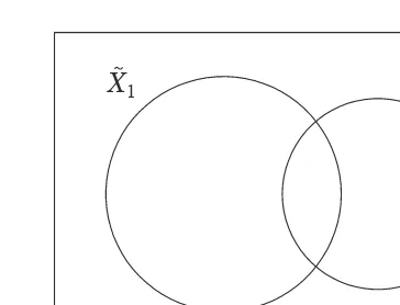
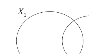
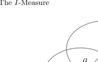
The relations between the (joint) entropies, conditional entropies, and mu-tual information for two random variablesX andY are given in Propositions 2.16 and 2.19. These relations can be summarized by the diagram in Figure 2.2 which is a variation of the Venn diagram4. One can check that all the rela-tions between Shannon’s information measures forX andY which are shown in Figure 2.2 are consistent with the relations given in Propositions 2.16 and 2.19. This one-to-one correspondence between Shannon’s information mea-sures and set theory is not just a coincidence for two random variables. We will discuss this in depth when we introduce the I-Measure in Chapter 3.

Analogous to entropy, there is a conditional version of mutual information called conditional mutual information.

4 _{The rectangle representing the universal set in a usual Venn diagram is missing}

(37)

2.2 Shannon’s Information Measures 17

H ( _X, _Y)

H ( _X| _Y) _H₍_Y|X₎

H ( _Y)

I ( _X; _Y)

H ( _X)

Fig. 2.2. Relationship between entropies and mutual information for two random variables.

Definition 2.20.For random variablesX,Y andZ, the mutual information between X andY conditioning on Z is defined as

I(X;Y_|Z) = X

x,y,z

p(x, y, z) log p(x, y|z)

p(x_|z)p(y_|z) =Elog

p(X, Y_|Z)

p(X_|Z)p(Y_|Z). (2.60)

Remark I(X;Y_|Z) is symmetrical inX andY.

Analogous to conditional entropy, we write

I(X;Y_|Z) =X

z

p(z)I(X;Y_|Z=z), (2.61)

where

I(X;Y_|Z=z) =X

x,y

p(x, y_|z) log p(x, y|z)

p(x_|z)p(y_|z). (2.62)

Similarly, when conditioning on two random variables, we write

I(X;Y|Z, T) =X

t

p(t)I(X;Y|Z, T =t) (2.63)

where

I(X;Y_|Z, T =t) = X

x,y,z

p(x, y, z_|t) log p(x, y|z, t)

p(x|z, t)p(y|z, t). (2.64)

(38)

Proposition 2.21.The mutual information between a random variable X

and itself conditioning on a random variable Z is equal to the conditional entropy ofX givenZ, i.e., I(X;X_|Z) =H(X_|Z).

Proposition 2.22.

I(X;Y|Z) =H(X|Z)−H(X|Y, Z), (2.65)

I(X;Y_|Z) =H(Y_|Z)₋H(Y_|X, Z), (2.66)

and

I(X;Y_|Z) =H(X_|Z) +H(Y_|Z)₋H(X, Y_|Z), (2.67)

provided that all the conditional entropies are finite.

Remark All Shannon’s information measures are finite if the random vari-ables involved have finite alphabets. Therefore, Propositions 2.19 and 2.22 apply provided that all the random variables therein have finite alphabets.

To conclude this section, we show that all Shannon’s information measures are special cases of conditional mutual information. Let Φ be a degenerate random variable, i.e., Φ takes a constant value with probability 1. Consider the mutual informationI(X;Y|Z). WhenX =Y andZ =Φ,I(X;Y|Z) be-comes the entropyH(X). WhenX =Y,I(X;Y|Z) becomes the conditional entropy H(X|Z). WhenZ =Φ, I(X;Y|Z) becomes the mutual information

I(X;Y). Thus all Shannon’s information measures are special cases of condi-tional mutual information.

2.3 Continuity of Shannon’s Information Measures for

Fixed Finite Alphabets

In this section, we prove that for fixed finite alphabets, all Shannon’s infor-mation measures are continuous functionals of the joint distribution of the random variables involved. To formulate the notion of continuity, we first introduce the variational distance5 _{as a distance measure between two}

prob-ability distributions on a common alphabet.

Definition 2.23.Let p and q be two probability distributions on a common alphabet _X. The variational distance betweenpandqis defined as

V(p, q) = X

x∈X

|p(x)₋q(x)_|. (2.68)

(39)

2.3 Continuity of Shannon’s Information Measures for Fixed Finite Alphabets 19

For a fixed finite alphabetX, letPX be the set of all distributions onX.

Then according to (2.35), the entropy of a distributionpon an alphabetX is defined as

H(p) =₋ X

x∈Sp

p(x) logp(x) (2.69)

where Sp denotes the support of p and Sp ⊂ X. In order for H(p) to be

continuous with respect to convergence in variational distance6 _{at a particular}

distributionp∈ PX, for anyǫ >0, there existsδ >0 such that

|H(p)₋H(q)_|< ǫ (2.70)

for allq∈ PX satisfying

V(p, q)< δ, (2.71)

or equivalently,

lim

p′_→_pH(p ′_{) =}_H

lim

p′_→_pp ′

=H(p), (2.72)

where the convergencep′ _→_p_{is in variational distance.}

Sincealoga_→0 asa_→0, we define a functionl: [0,_∞)_{→ ℜ}by

l(a) =

alogaifa >0

0 ifa= 0, (2.73)

i.e.,l(a) is a continuous extension ofaloga. Then (2.69) can be rewritten as

H(p) =₋X

x∈X

l(p(x)), (2.74)

where the summation above is over allxin X instead ofSp. Upon defining a

functionlx:PX → ℜfor allx∈ X by

lx(p) =l(p(x)), (2.75)

(2.74) becomes

H(p) =₋X

x∈X

lx(p). (2.76)

Evidently,lx(p) is continuous inp(with respect to convergence in variational

distance). Since the summation in (2.76) involves a finite number of terms, we conclude thatH(p) is a continuous functional ofp.

We now proceed to prove the continuity of conditional mutual information which covers all cases of Shannon’s information measures. ConsiderI(X;Y_|Z) and letpXY Z be the joint distribution ofX,Y, andZ, where the alphabets X,Y, and Z are assumed to be finite. From (2.47) and (2.67), we obtain

I(X;Y_|Z) =H(X, Z) +H(Y, Z)₋H(X, Y, Z)₋H(Z). (2.77)

(40)

Note that each term on the right hand side above is the unconditional entropy of the corresponding marginal distribution. Then (2.77) can be rewritten as

IX;Y|Z(pXY Z) =H(pXZ) +H(pY Z)−H(pXY Z)−H(pZ), (2.78)

It can readily be proved, for example, that

lim

by the continuity of H(·) when the alphabets involved are fixed and finite. The details are left as an exercise. Hence, we conclude that

lim

Since conditional mutual information covers all cases of Shannon’s infor-mation measures, we have proved that all Shannon’s inforinfor-mation measures are continuous with respect to convergence in variational distance under the assumption that the alphabets are fixed and finite. It is not difficult to show that under this assumption, convergence in variational distance is equivalent to_L2_{-convergence, i.e., convergence in Euclidean distance (see Problem 8). It}

follows that Shannon’s information measures are also continuous with respect to_L2_{-convergence. The variational distance, however, is more often used as a}

(41)

2.4 Chain Rules 21

2.4 Chain Rules

In this section, we present a collection of information identities known as the chain rules which are often used in information theory.

Proposition 2.24 (Chain Rule for Entropy).

H(X1, X2,· · ·, Xn) = n

X

i=1

H(Xi|X1,· · ·, Xi−1). (2.85)

Proof. The chain rule for n = 2 has been proved in Proposition 2.16. We prove the chain rule by induction on n. Assume (2.85) is true for n = m, wherem≥2. Then

H(X1,· · ·, Xm, Xm+1)

=H(X1,· · ·, Xm) +H(Xm+1|X1,· · ·, Xm) (2.86)

=

m

X

i=1

H(Xi|X1,· · ·, Xi−1) +H(Xm+1|X1,· · ·, Xm) (2.87)

=

m+1

X

i=1

H(Xi|X1,· · ·, Xi−1), (2.88)

where in (2.86) we have used (2.47) by letting X = (X1,· · ·, Xm) andY =

Xm+1, and in (2.87) we have used (2.85) for n = m. This proves the chain

rule for entropy. _⊓_⊔

The chain rule for entropy has the following conditional version.

Proposition 2.25 (Chain Rule for Conditional Entropy).

H(X1, X2,· · ·, Xn|Y) = n

X

i=1

H(Xi|X1,· · ·, Xi−1, Y). (2.89)

Proof. The proposition can be proved by considering

H(X1, X2,· · ·, Xn|Y)

=H(X1, X2,· · ·, Xn, Y)−H(Y) (2.90)

=H((X1, Y), X2,· · ·, Xn)−H(Y) (2.91)

=H(X1, Y) +

n

X

i=2

H(Xi|X1,· · ·, Xi−1, Y)−H(Y) (2.92)

=H(X1|Y) +

n

X

i=2

H(Xi|X1,· · ·, Xi−1, Y) (2.93)

=

n

X

i=1

(42)

where (2.90) and (2.93) follow from Proposition 2.16, while (2.92) follows from Proposition 2.24.

Alternatively, the proposition can be proved by considering

H(X1, X2,· · ·, Xn|Y)

where (2.95) and (2.98) follow from (2.43) and (2.45), respectively, and (2.96) follows from an application of Proposition 2.24 to the joint distribution of

X1, X2,· · ·, Xn conditioning on{Y =y}. This proof offers an explanation to

the observation that (2.89) can be obtained directly from (2.85) by condition-ing onY in every term. _⊓_⊔

Proposition 2.26 (Chain Rule for Mutual Information).

I(X1, X2,· · ·, Xn;Y) =

where in (2.101), we have invoked both Propositions 2.24 and 2.25. The chain rule for mutual information is proved. ⊓⊔

Proposition 2.27 (Chain Rule for Conditional Mutual Information).

(43)

2.5 Informational Divergence 23

Proof. This is the conditional version of the chain rule for mutual information. The proof is similar to that for Proposition 2.25. The details are omitted. ⊓⊔

2.5 Informational Divergence

Let pand q be two probability distributions on a common alphabet _X. We very often want to measure how muchpis different fromq, and vice versa. In order to be useful, this measure must satisfy the requirements that it is always nonnegative and it takes the zero value if and only if p=q. We denote the support ofpand qby _Sp andSq, respectively. Theinformational divergence

defined below serves this purpose.

Definition 2.28.The informational divergence between two probability dis-tributions pandqon a common alphabet _X is defined as

D(pkq) =X

x

p(x) logp(x)

q(x) =Eplog

p(X)

q(X), (2.104)

whereEp denotes expectation with respect top.

In the above definition, in addition to the convention that the summation is taken over Sp, we further adopt the convention clogc₀ = ∞ for c > 0.

With this convention, ifD(pkq)<∞, thenp(x) = 0 wheneverq(x) = 0, i.e.,

Sp⊂ Sq.

In the literature, the informational divergence is also referred to asrelative entropyor theKullback-Leibler distance. We note thatD(p_kq) is not symmet-rical inpandq, so it is not a truemetricor “distance.” Moreover,D(_·k·) does not satisfy the triangular inequality (see Problem 14).

In the rest of the book, the informational divergence will be referred to as divergencefor brevity. Before we prove that divergence is always nonnegative, we first establish the following simple but important inequality called the fundamental inequalityin information theory.

Lemma 2.29 (Fundamental Inequality). For anya >0,

lna_≤a₋1 (2.105)

with equality if and only if a= 1.

Proof. Let f(a) = lna₋a+ 1. Then f′₍_a_{) = 1}_/a₋_{1 and}_f′′₍_a_{) =} ₋₁_/a2_.

Since f(1) = 0, f′_{(1) = 0, and} _f′′_{(1) =} ₋₁ _< _{0, we see that} _f₍_a_{) attains}

(44)

!0.5 0 0.5 1 1.5 2 2.5 3

!1.5

!1

!0.5 0 0.5 1 1.5

1 _a

!1 a

ln a

Fig. 2.3.The fundamental inequality lna≤a−1.

Corollary 2.30.For any a >0,

lna_≥1₋1

a (2.106)

with equality if and only if a= 1.

Proof. This can be proved by replacingaby 1/a in (2.105). _⊓_⊔

We can see from Figure 2.3 that the fundamental inequality results from the convexity of the logarithmic function. In fact, many important results in information theory are also direct or indirect consequences of the convexity of the logarithmic function!

Theorem 2.31 (Divergence Inequality).For any two probability distribu-tionspandq on a common alphabet_X,

D(pkq)≥0 (2.107)

with equality if and only if p=q.

Proof. If q(x) = 0 for some x _{∈ S}p, then D(pkq) = ∞ and the theorem is

trivially true. Therefore, we assume thatq(x)>0 for allx∈ Sp. Consider

D(p_kq) = (loge)X

x∈Sp

p(x) lnp(x)

q(x) (2.108)

≥(loge)X

x∈Sp

p(x)

1₋q(x)

p(x)

(2.109)

= (loge)



X

x∈Sp

p(x)₋ X

x∈Sp

q(x)



 (2.110)

(45)

2.5 Informational Divergence 25

where (2.109) results from an application of (2.106), and (2.111) follows from

X

For equality to hold in (2.107), equality must hold in (2.109) for allx∈ Sp

and also in (2.111). For the former, we see from Lemma 2.29 that this is the case if and only if

p(x) =q(x) for allx∈ Sp, (2.113)

i.e., (2.111) holds with equality. Thus (2.113) is a necessary and sufficient condition for equality to hold in (2.107).

It is immediate that p = q implies (2.113), so it remains to prove the converse. SinceP_xq(x) = 1 andq(x)≥0 for allx,p(x) =q(x) for allx∈ Sp

impliesq(x) = 0 for allx6∈ Sp, and therefore p=q. The theorem is proved. ⊓

⊔

We now prove a very useful consequence of the divergence inequality called thelog-sum inequality.

Theorem 2.32 (Log-Sum Inequality).For positive numbersa1, a2,· · ·and

nonnegative numbers b1, b2,· · · such thatPiai<∞and0<Pibi<∞,

with the convention that logai₀ =_∞. Moreover, equality holds if and only if

ai

bi =constant for alli.

The log-sum inequality can easily be understood by writing it out for the case when there are two terms in each of the summations:

a1log {b′i}are probability distributions. Using the divergence inequality, we have

(46)

which implies (2.115). Equality holds if and only ifa′i =b′i for alli, or aibi =

constant for alli. The theorem is proved. ⊓⊔

One can also prove the divergence inequality by using the log-sum in-equality (see Problem 20), so the two inequalities are in fact equivalent. The log-sum inequality also finds application in proving the next theorem which gives a lower bound on the divergence between two probability distributions on a common alphabet in terms of the variational distance between them. We will see further applications of the log-sum inequality when we discuss the convergence of some iterative algorithms in Chapter 9.

Theorem 2.33 (Pinsker’s Inequality).

D(p_kq)_≥ 1 2 ln 2V

2₍_{p, q}₎_. _(2.120)

Both divergence and the variational distance can be used as measures of the difference between two probability distributions defined on the same al-phabet. Pinsker’s inequality has the important implication that for two proba-bility distributionspandqdefined on the same alphabet, ifD(p_kq) orD(q_kp) is small, then so is V(p, q). Furthermore, for a sequence of probability distri-butions qk, as k → ∞, ifD(pkqk)→ 0 orD(qkkp) →0, then V(p, qk)→ 0.

In other words, convergence in divergence is a stronger notion of convergence than convergence in variational distance.

The proof of Pinsker’s inequality as well as its consequence discussed above is left as an exercise (see Problems 23 and 24).

2.6 The Basic Inequalities

In this section, we prove that all Shannon’s information measures, namely entropy, conditional entropy, mutual information, and conditional mutual in-formation are always nonnegative. By this, we mean that these quantities are nonnegative for all joint distributions for the random variables involved.

Theorem 2.34.For random variablesX,Y, andZ,

I(X;Y|Z)≥0, (2.121)

with equality if and only if X and Y are independent when conditioning on

Z.

(47)

2.6 The Basic Inequalities 27

I(X;Y|Z)

= X

x,y,z

p(x, y, z) log p(x, y|z)

p(x_|z)p(y_|z) (2.122)

=X

z

p(z)X

x,y

p(x, y|z) log p(x, y|z)

p(x_|z)p(y_|z) (2.123)

=X

z

p(z)D(pXY|zkpX|zpY|z), (2.124)

where we have used pXY|z to denote {p(x, y|z),(x, y) ∈ X × Y}, etc. Since

for a fixed z, bothpXY|z andpX|zpY|z are joint probability distributions on X × Y, we have

D(pXY|zkpX|zpY|z)≥0. (2.125)

Therefore, we conclude thatI(X;Y_|Z)_≥0. Finally, we see from Theorem 2.31 that I(X;Y_|Z) = 0 if and only if for allz_{∈ S}z,

p(x, y_|z) =p(x_|z)p(y_|z), (2.126)

or

p(x, y, z) =p(x, z)p(y_|z) (2.127)

for allxandy. Therefore,X andY are independent conditioning onZ. The proof is accomplished. _⊓_⊔

As we have seen in Section 2.2 that all Shannon’s information measures are special cases of conditional mutual information, we already have proved that all Shannon’s information measures are always nonnegative. The nonneg-ativity of all Shannon’s information measures is called thebasic inequalities.

For entropy and conditional entropy, we offer the following more direct proof for their nonnegativity. Consider the entropyH(X) of a random variable

X. For allx_{∈ S}X, since 0< p(x)≤1, logp(x)≤0. It then follows from the

definition in (2.35) that H(X)_≥0. For the conditional entropy H(Y_|X) of random variableY given random variableX, sinceH(Y_|X =x)_≥0 for each

x_{∈ S}X, we see from (2.43) that H(Y|X)≥0.

Proposition 2.35.H(X) = 0if and only if X is deterministic.

Proof. If X is deterministic, i.e., there exists x∗ ∈ X such that p(x∗) = 1 and p(x) = 0 for all x 6= x∗, then H(X) = −p(x∗) logp(x∗) = 0. On the other hand, if X is not deterministic, i.e., there exists x∗ ∈ X such that 0 < p(x∗₎_< _{1, then} _H₍_X₎_{≥ −}_p₍_x∗_{) log}_p₍_x∗₎ _>_{0. Therefore, we conclude}

that H(X) = 0 if and only ifX is deterministic. _⊓_⊔

Proposition 2.36.H(Y_|X) = 0 if and only ifY is a function of X.

Proof. From (2.43), we see thatH(Y|X) = 0 if and only ifH(Y|X=x) = 0 for eachx∈ SX. Then from the last proposition, this happens if and only if

(48)

Proposition 2.37.I(X;Y) = 0if and only if X andY are independent.

Proof. This is a special case of Theorem 2.34 with Z being a degenerate random variable. _⊓_⊔

One can regard (conditional) mutual information as a measure of (con-ditional) dependency between two random variables. When the (con(con-ditional) mutual information is exactly equal to 0, the two random variables are (con-ditionally) independent.

We refer to inequalities involving Shannon’s information measures only (possibly with constant terms) asinformation inequalities. The basic inequal-ities are important examples of information inequalinequal-ities. Likewise, we refer to identities involving Shannon’s information measures only asinformation iden-tities. From the information identities (2.47), (2.57), and (2.65), we see that all Shannon’s information measures can be expressed as linear combinations of entropies provided that the latter are all finite. Specifically,

H(Y|X) =H(X, Y)−H(X), (2.128)

I(X;Y) =H(X) +H(Y)₋H(X, Y), (2.129)

and

I(X;Y|Z) =H(X, Z) +H(Y, Z)−H(X, Y, Z)−H(Z). (2.130)

Therefore, an information inequality is an inequality which involves only en-tropies.

As we will see later in the book, information inequalities form the most important set of tools for proving converse coding theorems in information theory. Except for a number of so-called non-Shannon-type inequalities, all known information inequalities are implied by the basic inequalities. Infor-mation inequalities will be studied systematically in Chapters 13, 14, and 15. In the next section, we will prove some consequences of the basic inequalities which are often used in information theory.

2.7 Some Useful Information Inequalities

In this section, we prove some useful consequences of the basic inequalities introduced in the last section. Note that the conditional versions of these inequalities can be proved by techniques similar to those used in the proof of Proposition 2.25.

Theorem 2.38 (Conditioning Does Not Increase Entropy).

H(Y_|X)_≤H(Y) (2.131)

(49)

2.7 Some Useful Information Inequalities 29

Proof. This can be proved by considering

H(Y_|X) =H(Y)₋I(X;Y)_≤H(Y), (2.132)

where the inequality follows becauseI(X;Y) is always nonnegative. The in-equality is tight if and only if I(X;Y) = 0, which is equivalent by Proposi-tion 2.37 toX andY being independent. _⊓_⊔

Similarly, it can be shown that

H(Y_|X, Z)_≤H(Y_|Z), (2.133)

which is the conditional version of the above proposition. These results have the following interpretation. SupposeY is a random variable we are interested in, andX andZare side-information aboutY. Then our uncertainty aboutY

cannot be increased on the average upon receiving side-informationX. Once we knowX, our uncertainty aboutY again cannot be increased on the average upon further receiving side-informationZ.

Remark Unlike entropy, the mutual information between two random vari-ables can be increased by conditioning on a third random variable. We refer the reader to Section 3.4 for a discussion.

Theorem 2.39 (Independence Bound for Entropy).

H(X1, X2,· · ·, Xn)≤ n

X

i=1

H(Xi) (2.134)

with equality if and only if Xi,i= 1,2,· · ·, nare mutually independent.

Proof. By the chain rule for entropy,

H(X1, X2,· · ·, Xn) = n

X

i=1

H(Xi|X1,· · ·, Xi−1) (2.135)

≤ n

X

i=1

H(Xi), (2.136)

where the inequality follows because we have proved in the last theorem that conditioning does not increase entropy. The inequality is tight if and only if it is tight for eachi, i.e.,

H(Xi|X1,· · ·, Xi−1) =H(Xi) (2.137)

for 1_≤i_≤n. From the last theorem, this is equivalent toXi being

(50)

p(x1, x2,· · ·, xn)

=p(x1, x2,· · ·, xn−1)p(xn) (2.138)

=p(p(x1, x2,· · ·, xn−2)p(xn−1)p(xn) (2.139)

.. .

=p(x1)p(x2)· · ·p(xn) (2.140)

for allx1, x2,· · ·, xn, i.e.,X1, X2,· · ·, Xn are mutually independent.

Alternatively, we can prove the theorem by considering

n

X

i=1

H(Xi)−H(X1, X2,· · ·, Xn)

=₋

n

X

i=1

Elogp(Xi) +Elogp(X1, X2,· · ·, Xn) (2.141)

=₋Elog[p(X1)p(X2)· · ·p(Xn)] +Elogp(X1, X2,· · ·, Xn) (2.142)

=Elog p(X1, X2,· · ·, Xn)

p(X1)p(X2)· · ·p(Xn)

(2.143)

=D(pX1X2···XnkpX1pX2· · ·pXn) (2.144)

≥0, (2.145)

where equality holds if and only if

p(x1, x2,· · ·, xn) =p(x1)p(x2)· · ·p(xn) (2.146)

for allx1, x2,· · ·, xn, i.e.,X1, X2,· · ·, Xn are mutually independent. ⊓⊔ Theorem 2.40.

I(X;Y, Z)_≥I(X;Y), (2.147)

with equality if and only if X_→Y _→Z forms a Markov chain.

Proof. By the chain rule for mutual information, we have

I(X;Y, Z) =I(X;Y) +I(X;Z|Y)≥I(X;Y). (2.148)

The above inequality is tight if and only if I(X;Z_|Y) = 0, orX _→Y _→Z

forms a Markov chain. The theorem is proved. _⊓_⊔

Lemma 2.41.If X_→Y _→Z forms a Markov chain, then

I(X;Z)≤I(X;Y) (2.149)

and

(51)

2.7 Some Useful Information Inequalities 31

Before proving this inequality, we first discuss its meaning. Suppose X

is a random variable we are interested in, and Y is an observation of X. If we inferX viaY, our uncertainty about X on the average is H(X_|Y). Now suppose we processY (either deterministically or probabilistically) to obtain a random variable Z. If we inferX viaZ, our uncertainty aboutX on the average isH(X_|Z). Since X _→Y _→Z forms a Markov chain, from (2.149), we have

H(X_|Z) =H(X)₋I(X;Z) (2.151)

≥H(X)−I(X;Y) (2.152)

=H(X_|Y), (2.153)

i.e., further processing ofY can only increase our uncertainty aboutX on the average.

Proof of Lemma 2.41. AssumeX_→Y _→Z, i.e.,X _⊥Z_|Y. By Theorem 2.34, we have

I(X;Z|Y) = 0. (2.154)

Then

I(X;Z) =I(X;Y, Z)₋I(X;Y_|Z) (2.155)

≤I(X;Y, Z) (2.156)

=I(X;Y) +I(X;Z|Y) (2.157)

=I(X;Y). (2.158)

In (2.155) and (2.157), we have used the chain rule for mutual information. The inequality in (2.156) follows because I(X;Y_|Z) is always nonnegative, and (2.158) follows from (2.154). This proves (2.149).

Since X _→ Y _→ Z is equivalent to Z _→ Y _→ X, we also have proved (2.150). This completes the proof of the lemma. _⊓_⊔

From Lemma 2.41, we can prove the more general data processing theorem.

Theorem 2.42 (Data Processing Theorem).If U _→X _→Y _→V forms a Markov chain, then

I(U;V)_≤I(X;Y). (2.159)

Proof. Assume U →X →Y →V. Then by Proposition 2.10, we have U →

X →Y andU →Y →V. From the first Markov chain and Lemma 2.41, we have

I(U;Y)≤I(X;Y). (2.160) From the second Markov chain and Lemma 2.41, we have

I(U;V)≤I(U;Y). (2.161)

(52)

2.8 Fano’s Inequality

In the last section, we have proved a few information inequalities involving only Shannon’s information measures. In this section, we first prove an upper bound on the entropy of a random variable in terms of the size of the alpha-bet. This inequality is then used in the proof of Fano’s inequality, which is extremely useful in proving converse coding theorems in information theory.

Theorem 2.43.For any random variableX,

H(X)_≤log_{|X |}, (2.162)

where_{|X |}denotes the size of the alphabet_X. This upper bound is tight if and only ifX is distributed uniformly on _X.

Proof. Let u be the uniform distribution on X, i.e., u(x) = |X |−1 _{for all}

x∈ X. Then

log_{|X | −}H(X)

=− X

x∈SX

p(x) log|X |−1₊ X

x∈SX

p(x) logp(x) (2.163)

=₋ X

x∈SX

p(x) logu(x) + X

x∈SX

p(x) logp(x) (2.164)

= X

x∈SX

p(x) log p(x)

u(x) (2.165)

=D(pku) (2.166)

≥0, (2.167)

proving (2.162). This upper bound is tight if and if only D(pku) = 0, which from Theorem 2.31 is equivalent top(x) =u(x) for allx∈ X, completing the proof. ⊓⊔

Corollary 2.44.The entropy of a random variable may take any nonnegative real value.

Proof. Consider a random variable X defined on a fixed finite alphabet _X. We see from the last theorem that H(X) = log_{|X |} is achieved when X is distributed uniformly on_X. On the other hand,H(X) = 0 is achieved when

X is deterministic. For 0_≤a_{≤ |X |}−1_{, let}

g(a) =H(_{1₋(_{|X | −}1)a, a,_{· · ·}, a_}) (2.168) =−l(1−(|X | −1)a)−(|X | −1)l(a), (2.169)

wherel(_·) is defined in (2.73). Note thatg(a) is continuous ina, withg(0) = 0 and g(_{|X |}−1_{) = log}