Data Analysis Cookbook Recipes Deliver 8675 pdf pdf

(1)

(2)

R Data Analysis

Cookbook

Over 80 recipes to help you breeze through your

data analysis projects using R

Viswa Viswanathan

Shanthi Viswanathan

(3)

R Data Analysis Cookbook

All rights reserved. No part of this book may be reproduced, stored in a retrieval system, or transmitted in any form or by any means, without the prior written permission of the publisher, except in the case of brief quotations embedded in critical articles or reviews. Every effort has been made in the preparation of this book to ensure the accuracy of the information presented. However, the information contained in this book is sold without warranty, either express or implied. Neither the authors, nor Packt Publishing, and its dealers and distributors will be held liable for any damages caused or alleged to be caused directly or indirectly by this book.

Packt Publishing has endeavored to provide trademark information about all of the companies and products mentioned in this book by the appropriate use of capitals. However, Packt Publishing cannot guarantee the accuracy of this information.

First published: May 2015

Production reference: 1220515

Published by Packt Publishing Ltd. Livery Place

35 Livery Street

Birmingham B3 2PB, UK. ISBN 978-1-78398-906-5

(4)

(5)

About the Authors

Viswa Viswanathan is an associate professor of Computing and Decision Sciences at

the Stillman School of Business in Seton Hall University. After completing his PhD in artificial intelligence, Viswa spent a decade in academia and then switched to a leadership position in the software industry for a decade. During this period, he worked for Infosys, Igate, and Starbase. He embraced academia once again in 2001.

Viswa has taught extensively in fields ranging from operations research, computer science, software engineering, management information systems, and enterprise systems. In addition to teaching at the university, Viswa has conducted training programs for industry professionals. He has written several peer-reviewed research publications in journals such as Operations Research, IEEE Software, Computers and Industrial Engineering, and International Journal of Artificial Intelligence in Education. He has authored a book titled Data Analytics with R: A hands-on approach.

Viswa thoroughly enjoys hands-on software development, and has single-handedly conceived, architected, developed, and deployed several web-based applications.

Apart from his deep interest in technical fields such as data analytics, artificial intelligence, computer science, and software engineering, Viswa harbors a deep interest in education, with special emphasis on the roots of learning and methods to foster deeper learning. He has done research in this area and hopes to pursue the subject further.

(6)

Shanthi Viswanathan is an experienced technologist who has delivered technology

management and enterprise architecture consulting to many enterprise customers. She has worked for Infosys Technologies, Oracle Corporation, and Accenture. As a consultant, Shanthi has helped several large organizations, such as Canon, Cisco, Celgene, Amway, Time Warner Cable, and GE among others, in areas such as data architecture and analytics, master data management, service-oriented architecture, business process management, and modeling. When she is not in front of her Mac, Shanthi spends time hiking in the suburbs of NY/NJ, working in the garden, and teaching yoga.

(7)

About the Reviewers

Kenneth D. Graves believes that data science will give us superpowers. Or, at the

very least, allow us to make better decisions. Toward this end, he has over 15 years of experience in data science and technology, specializing in machine learning, big data, signal processing and marketing, and social media analytics. He has worked for Fortune 500 companies such as CBS and RCA-Technicolor, as well as finance and technology companies, designing state-of-art technologies and data solutions to improve business and organizational decision-making processes and outcomes. His projects have included facial and brand recognition, natural language processing, and predictive analytics. He works and mentors others in many technologies, including R, Python, C++, Hadoop, and SQL.

Kenneth holds degrees and/or certifications in data science, business, film, and classical languages. When he is not trying to discover superpowers, he is a data scientist and acting CTO at Soshag, LLC., a social media analytics firm. He is available for consulting and data science projects throughout the Greater Boston Area. He currently lives in Wellesley, MA.

I wish to thank my wife, Jill, for being the inspiration for all that I do.

Jithin S L completed his BTech in information technology from Loyola Institute of Technology

and Science. He started his career in the field of analytics and then moved to various verticals of big data technology. He has worked with reputed organizations, such as Thomson Reuters, IBM, and Flytxt, in different roles. He has worked in the banking, energy, healthcare, and telecom domains, and has handled global projects on big data technology.

(8)

provides an opportunity to learn new things in a new way, experiment, explore, and advise towards success.”

-Jithin

I surrender myself to God almighty who helped me review this book in an effective way. I dedicate my work on this book to my dad, Mr. N. Subbian Asari; my lovable mom, Mrs. M. Lekshmi; and my sweet sister, Ms. S.L Jishma, for coordinating and encouraging me to review this book. Last but not least, I would like to thank all my friends.

Dipanjan Sarkar is an IT engineer at Intel, the world's largest silicon company, where he

works on analytics and enterprise application development. As part of his experience in the industry so far, he has previously worked as a data engineer at DataWeave, one of India's emerging big data analytics start-ups and also as a graduate technical intern in Intel. Dipanjan received his master's degree in information technology from the International Institute of Information Technology, Bengaluru. His interests include learning about new technology, disruptive start-ups, and data science. He has also reviewed Learning R for Geospatial Analysis, Packt Publishing.

Hang (Harvey) Yu graduated from the University of Illinois at Urbana-Champaign with

a PhD in computational biophysics and a master's degree in statistics. He has extensive experience on data mining, machine learning, and statistics. In the past, Harvey has worked on areas such as stochastic simulations and time series (in C and Python) as part of his academic work. He was intrigued by algorithms and mathematical modeling. He has been involved in data analytics since then.

He is currently working as a data scientist in Silicon Valley. He is passionate about data sciences. He has developed statistical/mathematical models based on techniques such as optimization and predictive modeling in R. Previously, Harvey worked as a computational sciences intern for ExxonMobil.

(9)

www.PacktPub.com

Support files, eBooks, discount offers, and more

For support files and downloads related to your book, please visit www.PacktPub.com.

Did you know that Packt offers eBook versions of every book published, with PDF and ePub files available? You can upgrade to the eBook version at www.PacktPub.com and as a print book customer, you are entitled to a discount on the eBook copy. Get in touch with us at

service@packtpub.com for more details.

At www.PacktPub.com, you can also read a collection of free technical articles, sign up for a range of free newsletters and receive exclusive discounts and offers on Packt books and eBooks.

TM

https://www2.packtpub.com/books/subscription/packtlib

Do you need instant solutions to your IT questions? PacktLib is Packt's online digital book library. Here, you can search, access, and read Packt's entire library of books.

Why Subscribe?

f Fully searchable across every book published by Packt f Copy and paste, print, and bookmark content

f On demand and accessible via a web browser

Free Access for Packt account holders

(10)

Preface v

Chapter 1: Acquire and Prepare the Ingredients – Your Data

1

Introduction 2

Reading data from CSV files 2

Reading XML data 5 Reading JSON data 7

Reading data from fixed-width formatted files 8

Reading data from R files and R libraries 9

Removing cases with missing values 11 Replacing missing values with the mean 13 Removing duplicate cases 15

Rescaling a variable to [0,1] 16

Normalizing or standardizing data in a data frame 18

Binning numerical data 20

Creating dummies for categorical variables 22

Chapter 2: What's in There? – Exploratory Data Analysis

25

Introduction 26

Creating standard data summaries 26

Extracting a subset of a dataset 28

Splitting a dataset 31 Creating random data partitions 32

Generating standard plots such as histograms, boxplots, and scatterplots 35

Generating multiple plots on a grid 43 Selecting a graphics device 45

Creating plots with the lattice package 46

Creating plots with the ggplot2 package 49

Creating charts that facilitate comparisons 55

(11)

Table of Contents

Creating multivariate plots 62

Chapter 3:

Where Does It Belong? – Classification

65

Introduction 65

Generating error/classification-confusion matrices 66

Generating ROC charts 69

Building, plotting, and evaluating – classification trees 72

Using random forest models for classification 78

Classifying using the support vector machine approach 81

Classifying using the Naïve Bayes approach 85

Classifying using the KNN approach 88

Using neural networks for classification 90

Classifying using linear discriminant function analysis 93

Classifying using logistic regression 95

Using AdaBoost to combine classification tree models 98

Chapter 4:

Give Me a Number – Regression

101

Introduction 101

Computing the root mean squared error 102

Building KNN models for regression 104

Performing linear regression 110

Performing variable selection in linear regression 117

Building regression trees 120

Building random forest models for regression 127 Using neural networks for regression 132

Performing k-fold cross-validation 135

Performing leave-one-out-cross-validation to limit overfitting 137

Chapter 5:

Can You Simplify That? – Data Reduction Techniques

139

Introduction 139

Performing cluster analysis using K-means clustering 140

Performing cluster analysis using hierarchical clustering 146 Reducing dimensionality with principal component analysis 150

Chapter 6: Lessons from History – Time Series Analysis

159

Introduction 159

Creating and examining date objects 159

Operating on date objects 164

Performing preliminary analyses on time series data 166

Using time series objects 170

(12)

Table of Contents

Chapter 7:

It's All About Your Connections – Social Network Analysis 187

Introduction 187

Downloading social network data using public APIs 188

Creating adjacency matrices and edge lists 192

Plotting social network data 196

Computing important network metrics 209

Chapter 8:

Put Your Best Foot Forward – Document and Present

Your Analysis

217

Introduction 217

Generating reports of your data analysis with R Markdown and knitr 218

Creating interactive web applications with shiny 228

Creating PDF presentations of your analysis with R Presentation 234

Chapter 9: Work Smarter, Not Harder – Efficient and Elegant R Code 239

Introduction 239

Exploiting vectorized operations 240

Processing entire rows or columns using the apply function 242 Applying a function to all elements of a collection with lapply and sapply 245

Applying functions to subsets of a vector 248

Using the split-apply-combine strategy with plyr 250

Slicing, dicing, and combining data with data tables 253

Chapter 10: Where in the World? – Geospatial Analysis

261

Introduction 262

Downloading and plotting a Google map of an area 262

Overlaying data on the downloaded Google map 265

Importing ESRI shape files into R 267

Using the sp package to plot geographic data 270

Getting maps from the maps package 274 Creating spatial data frames from regular data frames containing

spatial and other data 275

Creating spatial data frames by combining regular data frames

with spatial objects 277

Adding variables to an existing spatial data frame 282

Chapter 11:

Playing Nice – Connecting to Other Systems

285

Introduction 285

Using Java objects in R 286

Using JRI to call R functions from Java 292

Using Rserve to call R functions from Java 295

Executing R scripts from Java 298

(13)

Table of Contents

Reading data from relational databases – MySQL 302

Reading data from NoSQL databases – MongoDB 307

(14)

Preface

Since the release of version 1.0 in 2000, R's popularity as an environment for statistical computing, data analytics, and graphing has grown exponentially. People who have been using spreadsheets and need to perform things that spreadsheet packages cannot readily do, or need to handle larger data volumes than what a spreadsheet program can comfortably handle, are looking to R. Analogously, people using powerful commercial analytics packages are also intrigued by this free and powerful option. As a result, a large number of people are now looking to quickly get things done in R.

Being an extensible system, R's functionality is divided across numerous packages with each one exposing large numbers of functions. Even experienced users cannot expect to remember all the details off the top of their head. This cookbook, aimed at users who are already exposed to the fundamentals of R, provides ready recipes to perform many important data analytics tasks. Instead of having to search the Web or delve into numerous books when faced with a specific task, people can find the appropriate recipe and get going in a matter of minutes.

What this book covers

Chapter 1, Acquire and Prepare the Ingredients – Your Data, covers the activities that precede the actual data analysis task. It provides recipes to read data from different input file formats. Furthermore, prior to actually analyzing the data, we perform several preparatory and data cleansing steps and the chapter also provides recipes for these: handling missing values and duplicates, scaling or standardizing values, converting between numerical and categorical variables, and creating dummy variables.

(15)

Preface

Chapter 3, Where Does It Belong? – Classification, covers recipes for applying classification techniques. It includes classification trees, random forests, support vector machines, Naïve Bayes, K-nearest neighbors, neural networks, linear and quadratic discriminant analysis, and logistic regression.

Chapter 4, Give Me a Number – Regression, is about recipes for regression techniques. It includes K-nearest neighbors, linear regression, regression trees, random forests, and neural networks.

Chapter 5, Can You Simplify That? – Data Reduction Techniques, covers recipes for data reduction. It presents cluster analysis through K-means and hierarchical clustering. It also covers principal component analysis.

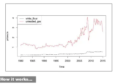
Chapter 6, Lessons from History – Time Series Analysis, coversrecipesto workwithdate and date/time objects, create and plot time-series objects, decompose, filter and smooth time series, and perform ARIMA analysis.

Chapter 7, It's All About Your Connections – Social Network Analysis, is aboutsocial networks. It includes recipes to acquire social network data using public APIs, create and plot social networks, and compute important network metrics.

Chapter 8, Put Your Best Foot Forward – Document and Present Your Analysis, considers techniques to disseminate your analysis. It includes recipes to use R markdown and KnitR to generate reports, to use shiny to create interactive applications that enable your audience to directly interact with the data, and to create presentations with RPres.

Chapter 9, Work Smarter, Not Harder – Efficient and Elegant R Code, addresses the issue of writing efficient and elegant R code in the context of handling large data. It covers recipes to use the apply family of functions, to use the plyr package, and to use data tables to slice and dice data.

Chapter 10, Where in the World? – Geospatial Analysis, covers the topic of exploiting R's powerful features to handle spatial data. It covers recipes to use RGoogleMaps to get GoogleMaps and to superimpose our own data on them, to import ESRI shape files into R and plot them, to import maps from the maps package, and to use the sp package to create and plot spatial data frame objects.

(16)

What you need for this book

We have tested all the code in this book for R versions 3.0.2 (Frisbee Sailing) and 3.1.0 (Spring Dance). When you install or load some of the packages, you may get a warning message to the effect that the code was compiled for a different version, but this will not impact any of the code in this book.

Who this book is for

This book is ideal for those who are already exposed to R, but have not yet used it extensively for data analytics and are seeking to get up and running quickly for analytics tasks. This book will help people who aspire to enhance their skills in any of the following ways:

f perform advanced analyses and create informative and professional charts f become proficient in acquiring data from many sources

f apply supervised and unsupervised data mining techniques f use R's features to present analyses professionally

Sections

In this book, you will find several headings that appear frequently (Getting ready, How to do it, How it works, There's more, and See also).

To give clear instructions on how to complete a recipe, we use these sections as follows:

Getting ready

This section tells you what to expect in the recipe, and describes how to set up any software or any preliminary settings required for the recipe.

How to do it…

This section contains the steps required to follow the recipe.

How it works…

(17)

Preface

There's more…

This section consists of additional information about the recipe in order to make the reader more knowledgeable about the recipe.

Conventions

In this book, you will find a number of text styles that distinguish between different kinds of information. Here are some examples of these styles and an explanation of their meaning. Code words in text, database table names, folder names, filenames, file extensions, pathnames, dummy URLs, user input, and Twitter handles are shown as follows: "The read.csv() function creates a data frame from the data in the .csv file."

A block of code is set as follows: > names(auto)

[1] "No" "mpg" "cylinders" [4] "displacement" "horsepower" "weight" [7] "acceleration" "model_year" "car_name"

Any command-line input or output is written as follows:

export LD_LIBRARY_PATH=$JAVA_HOME/jre/lib/server

export MAKEFLAGS="LDFLAGS=-Wl,-rpath $JAVA_HOME/lib/server"

New terms and important words are shown in bold. Words that you see on the screen, for example, in menus or dialog boxes, appear in the text like this: "Clicking the Next button moves you to the next screen."

(18)

Reader feedback

Feedback from our readers is always welcome. Let us know what you think about this book—what you liked or disliked. Reader feedback is important for us as it helps us develop titles that you will really get the most out of.

To send us general feedback, simply e-mail feedback@packtpub.com, and mention the book's title in the subject of your message.

If there is a topic that you have expertise in and you are interested in either writing or contributing to a book, see our author guide at www.packtpub.com/authors.

Customer support

Now that you are the proud owner of a Packt book, we have a number of things to help you to get the most from your purchase.

Downloading the example code and data

You can download the example code files from your account at http://www.packtpub.com

for all the Packt Publishing books you have purchased. If you purchased this book elsewhere, you can visit http://www.packtpub.com/support and register to have the files e-mailed

directly to you.

About the data files used in this book

We have generated many of the data files used in this book. We have also used some publicly available data sets. The table below lists the sources of these public data sets. We downloaded most of the public data sets from the University of California at Irvine (UCI) Machine Learning Repository at http://archive.ics.uci.edu/ml/. In the table below we have indicated this as "Downloaded from UCI-MLR."

Data file name Source

auto-mpg.csv Quinlan, R. Combining Instance-Based and Model-Based Learning, Machine Learning Proceedings on the Tenth International Conference 1993, 236-243, held at University of Massachusetts, Amherst published by Morgan Kaufmann.

(Downloaded from UCI-MLR).

BostonHousing. csv

(19)

Preface

daily-bike-rentals.csv

Fanaee-T, Hadi, and Gama, Joao, Event labeling combining ensemble detectors and background knowledge, Progress in Artificial Intelligence (2013): pp. 1-15, Springer Berlin Heidelberg. (Downloaded from UCI-MLR)

banknote-authentication. csv

f Owner of database: Volker Lohweg, University of Applied Sciences, Ostwestfalen-Lippe

f Donor of database: Helene Darksen, University of Applied Sciences, Ostwestfalen-Lippe

(Downloaded from UCI-MLR)

education.csv Robust Regression and Outlier Detection, P. J. Rouseeuw and A. M. Leroy, Wiley, 1987.

prices.csv Downloaded from the US Bureau of Labor Statistics.

infy.csv, infy-monthly.csv

Downloaded from Yahoo! Finance.

nj-wages.csv NJ Department of Education's website and

http://federalgovernmentzipcodes.us.

Downloading the color images of this book

(20)

Errata

Although we have taken every care to ensure the accuracy of our content, mistakes do happen. If you find a mistake in one of our books—maybe a mistake in the text or the code—we would be grateful if you could report this to us. By doing so, you can save other readers from frustration and help us improve subsequent versions of this book. If you find any errata, please report them by visiting http://www.packtpub.com/submit-errata, selecting your book, clicking on the ErrataSubmissionForm link, and entering the details of your errata. Once your errata are verified, your submission will be accepted and the errata will be uploaded to our website or added to any list of existing errata under the Errata section of that title.

To view the previously submitted errata, go to https://www.packtpub.com/books/ content/support and enter the name of the book in the search field. The required

information will appear under the Errata section.

Piracy

Piracy of copyrighted material on the Internet is an ongoing problem across all media. At Packt, we take the protection of our copyright and licenses very seriously. If you come across any illegal copies of our works in any form on the Internet, please provide us with the location address or website name immediately so that we can pursue a remedy.

Please contact us at copyright@packtpub.com with a link to the suspected pirated material. We appreciate your help in protecting our authors and our ability to bring you valuable content.

Questions

If you have a problem with any aspect of this book, you can contact us at

(21)

(22)

1

Acquire and Prepare

the Ingredients –

Your Data

In this chapter, we will cover:

f Reading data from CSV files

f Reading XML data f Reading JSON data

f Reading data from fixed-width formatted files

f Reading data from R data files and R libraries

f Removing cases with missing values f Replacing missing values with the mean f Removing duplicate cases

f Rescaling a variable to [0,1]

f Normalizing or standardizing data in a data frame f Binning numerical data

(23)

Acquire and Prepare the Ingredients – Your Data

Introduction

Data analysts need to load data from many different input formats into R. Although R has its own native data format, data usually exists in text formats, such as CSV (Comma Separated Values), JSON (JavaScript Object Notation), and XML (Extensible Markup Language). This chapter provides recipes to load such data into your R system for processing.

Very rarely can we start analyzing data immediately after loading it. Often, we will need to preprocess the data to clean and transform it before embarking on analysis. This chapter provides recipes for some common cleaning and preprocessing steps.

Reading data from CSV files

CSV formats are best used to represent sets or sequences of records in which each record has an identical list of fields. This corresponds to a single relation in a relational database, or to data (though not calculations) in a typical spreadsheet.

Getting ready

If you have not already downloaded the files for this chapter, do it now and ensure that the

auto-mpg.csv file is in your R working directory.

How to do it...

Reading data from .csv files can be done using the following commands:

1. Read the data from auto-mpg.csv, which includes a header row: > auto <- read.csv("auto-mpg.csv", header=TRUE, sep = ",")

2. Verify the results: > names(auto)

How it works...

The read.csv() function creates a data frame from the data in the .csv file. If we pass header=TRUE, then the function uses the very first row to name the variables in the resulting

data frame:

(24)

[4] "displacement" "horsepower" "weight" [7] "acceleration" "model_year" "car_name"

The header and sep parameters allow us to specify whether the .csv file has headers and

the character used in the file to separate fields. The header=TRUE and sep="," parameters are the defaults for the read.csv() function—we can omit these in the code example.

There's more...

The read.csv() function is a specialized form of read.table(). The latter uses whitespace as the default field separator. We discuss a few important optional arguments to these functions.

Handling different column delimiters

In regions where a comma is used as the decimal separator, .csv files use ";" as the field

delimiter. While dealing with such data files, use read.csv2() to load data into R.

Alternatively, you can use the read.csv("<file name>", sep=";", dec=",") command. Use sep="\t" for tab-delimited files.

Handling column headers/variable names

If your data file does not have column headers, set header=FALSE.

The auto-mpg-noheader.csv file does not include a header row. The first command in

the following snippet reads this file. In this case, R assigns default variable names V1, V2, and so on:

> auto <- read.csv("auto-mpg-noheader.csv", header=FALSE) > head(auto,2)

V1 V2 V3 V4 V5 V6 V7 V8 V9 1 1 28 4 140 90 2264 15.5 71 chevrolet vega 2300 2 2 19 3 70 97 2330 13.5 72 mazda rx2 coupe

If your file does not have a header row, and you omit the header=FALSE optional argument, the read.csv() function uses the first row for variable names and ends up constructing

variable names by adding X to the actual data values in the first row. Note the meaningless variable names in the following fragment:

> auto <- read.csv("auto-mpg-noheader.csv") > head(auto,2)

(25)

We can use the optional col.names argument to specify the column names. If col.names

is given explicitly, the names in the header row are ignored even if header=TRUE is specified:

> auto <- read.csv("auto-mpg-noheader.csv", header=FALSE, col.names =

c("No", "mpg", "cyl", "dis","hp", "wt", "acc", "year", "car_name"))

> head(auto,2)

No mpg cyl dis hp wt acc year car_name 1 1 28 4 140 90 2264 15.5 71 chevrolet vega 2300 2 2 19 3 70 97 2330 13.5 72 mazda rx2 coupe

Handling missing values

When reading data from text files, R treats blanks in numerical variables as NA (signifying missing data). By default, it reads blanks in categorical attributes just as blanks and not as

NA. To treat blanks as NA for categorical and character variables, set na.strings="":

> auto <- read.csv("auto-mpg.csv", na.strings="")

If the data file uses a specified string (such as "N/A" or "NA" for example) to indicate the missing values, you can specify that string as the na.strings argument, as in

na.strings= "N/A" or na.strings = "NA".

Reading strings as characters and not as factors

By default, R treats strings as factors (categorical variables). In some situations, you may want to leave them as character strings. Use stringsAsFactors=FALSE to achieve this:

> auto <- read.csv("auto-mpg.csv",stringsAsFactors=FALSE)

However, to selectively treat variables as characters, you can load the file with the defaults (that is, read all strings as factors) and then use as.character() to convert the requisite factor variables to characters.

Reading data directly from a website

If the data file is available on the Web, you can load it into R directly instead of downloading and saving it locally before loading it into R:

(26)

Reading XML data

You may sometimes need to extract data from websites. Many providers also supply data in XML and JSON formats. In this recipe, we learn about reading XML data.

Getting ready

If the XML package is not already installed in your R environment, install the package now as follows:

> install.packages("XML")

How to do it...

XML data can be read by following these steps: 1. Load the library and initialize:

> library(XML)

> url <- "http://www.w3schools.com/xml/cd_catalog.xml"

2. Parse the XML file and get the root node: > xmldoc <- xmlParse(url)

> rootNode <- xmlRoot(xmldoc) > rootNode[1]

3. Extract XML data:

> data <- xmlSApply(rootNode,function(x) xmlSApply(x, xmlValue))

4. Convert the extracted data into a data frame:

> cd.catalog <- data.frame(t(data),row.names=NULL)

5. Verify the results: > cd.catalog[1:2,]

How it works...

The xmlParse function returns an object of the XMLInternalDocument class, which is a C-level internal data structure.

The xmlRoot() function gets access to the root node and its elements. We check the first

(27)

To extract data from the root node, we use the xmlSApply() function iteratively over all the children of the root node. The xmlSApply function returns a matrix.

To convert the preceding matrix into a data frame, we transpose the matrix using the t()

function. We then extract the first two rows from the cd.catalog data frame: > cd.catalog[1:2,]

TITLE ARTIST COUNTRY COMPANY PRICE YEAR 1 Empire Burlesque Bob Dylan USA Columbia 10.90 1985 2 Hide your heart Bonnie Tyler UK CBS Records 9.90 1988

There's more...

XML data can be deeply nested and hence can become complex to extract. Knowledge of

XPath will be helpful to access specific XML tags. R provides several functions such as xpathSApply and getNodeSet to locate specific elements.

Extracting HTML table data from a web page

Though it is possible to treat HTML data as a specialized form of XML, R provides specific functions to extract data from HTML tables as follows:

> url <- "http://en.wikipedia.org/wiki/World_population" > tables <- readHTMLTable(url)

> world.pop <- tables[[5]]

The readHTMLTable() function parses the web page and returns a list of all tables that are found on the page. For tables that have an id attribute, the function uses the id attribute as the name of that list element.

We are interested in extracting the "10 most populous countries," which is the fifth table; hence we use tables[[5]].

(28)

Specify which to get data from a specific table. R returns a data frame.

Reading JSON data

Several RESTful web services return data in JSON format—in some ways simpler and more efficient than XML. This recipe shows you how to read JSON data.

Getting ready

R provides several packages to read JSON data, but we use the jsonlite package. Install

the package in your R environment as follows:

> install.packages("jsonlite")

students.json files and student-courses.json files are in your R working directory.

How to do it...

Once the files are ready and load the jsonlite package and read the files as follows:

1. Load the library:

> library(jsonlite)

2. Load the JSON data from files:

> dat.1 <- fromJSON("students.json")

> dat.2 <- fromJSON("student-courses.json")

3. Load the JSON document from the Web:

> url <- "http://finance.yahoo.com/webservice/v1/symbols/ allcurrencies/quote?format=json"

> jsonDoc <- fromJSON(url)

4. Extract data into data frames:

> dat <- jsonDoc$list$resources$resource$fields

5. Verify the results:

> dat[1:2,] > dat.1[1:3,]

(29)

How it works...

The jsonlite package provides two key functions: fromJSON and toJSON.

The fromJSON function can load data either directly from a file or from a web page as the preceding steps 2 and 3 show. If you get errors in downloading content directly from the Web, install and load the httr package.

Depending on the structure of the JSON document, loading the data can vary in complexity. If given a URL, the fromJSON function returns a list object. In the preceding list, in step 4, we see how to extract the enclosed data frame.

Reading data from fixed-width formatted

files

In fixed-width formatted files, columns have fixed widths; if a data element does not use up the entire allotted column width, then the element is padded with spaces to make up the specified width. To read fixed-width text files, specify columns by column widths or by starting positions.

Getting ready

Download the files for this chapter and store the student-fwf.txt file in your R

working directory.

How to do it...

Read the fixed-width formatted file as follows:

> student <- read.fwf("student-fwf.txt", widths=c(4,15,20,15,4),

col.names=c("id","name","email","major","year"))

How it works...

In the student-fwf.txt file, the first column occupies 4 character positions, the second

15, and so on. The c(4,15,20,15,4) expression specifies the widths of the five columns

in the data file.

(30)

There's more...

The read.fwf() function has several optional arguments that come in handy. We discuss a few of these as follows:

Files with headers

Files with headers use the following command:

> student <- read.fwf("student-fwf-header.txt", widths=c(4,15,20,15,4), header=TRUE, sep="\t",skip=2)

If header=TRUE, the first row of the file is interpreted as having the column headers. Column

headers, if present, need to be separated by the specified sep argument. The sep argument only applies to the header row.

The skip argument denotes the number of lines to skip; in this recipe, the first two lines are skipped.

Excluding columns from data

To exclude a column, make the column width negative. Thus, to exclude the e-mail column, we will specify its width as -20 and also remove the column name from the col.names

vector as follows:

> student <- read.fwf("student-fwf.txt",widths=c(4,15,-20,15,4), col.names=c("id","name","major","year"))

Reading data from R files and R libraries

During data analysis, you will create several R objects. You can save these in the native R data format and retrieve them later as needed.

Getting ready

First, create and save R objects interactively as shown in the following code. Make sure you have write access to the R working directory:

> customer <- c("John", "Peter", "Jane")

> orderdate <- as.Date(c('2014-10-1','2014-1-2','2014-7-6')) > orderamount <- c(280, 100.50, 40.25)

> order <- data.frame(customer,orderdate,orderamount) > names <- c("John", "Joan")

(31)

After saving the preceding code, the remove() function deletes the object from the current session.

How to do it...

To be able to read data from R files and libraries, follow these steps:

1. Load data from R data files into memory: > load("test.Rdata")

> ord <- readRDS("order.rds")

2. The datasets package is loaded in the R environment by default and contains

the iris and cars datasets. To load these datasets' data into memory, use the

following code:

> data(iris)

> data(c(cars,iris))

The first command loads only the iris dataset, and the second loads the cars and

iris datasets.

How it works...

The save() function saves the serialized version of the objects supplied as arguments along with the object name. The subsequent load() function restores the saved objects with the same object names they were saved with, to the global environment by default. If there are existing objects with the same names in that environment, they will be replaced without any warnings.

The saveRDS() function saves only one object. It saves the serialized version of the object and not the object name. Hence, with the readRDS() function the saved object can be restored into a variable with a different name from when it was saved.

There's more...

The preceding recipe has shown you how to read saved R objects. We see more options in this section.

To save all objects in a session

The following command can be used to save all objects:

(32)

To selectively save objects in a session

To save objects selectively use the following commands: > odd <- c(1,3,5,7)

> even <- c(2,4,6,8)

> save(list=c("odd","even"),file="OddEven.Rdata")

The list argument specifies a character vector containing the names of the objects to be

saved. Subsequently, loading data from the OddEven.Rdata file creates both odd and even

objects. The saveRDS() function can save only one object at a time.

Attaching/detaching R data files to an environment

While loading Rdata files, if we want to be notified whether objects with the same name

already exist in the environment, we can use: > attach("order.Rdata")

The order.Rdata file contains an object named order. If an object named order already exists in the environment, we will get the following error:

The following object is masked _by_ .GlobalEnv:

order

Listing all datasets in loaded packages

All the loaded packages can be listed using the following command: > data()

Removing cases with missing values

Datasets come with varying amounts of missing data. When we have abundant data, we sometimes (not always) want to eliminate the cases that have missing values for one or more variables. This recipe applies when we want to eliminate cases that have any missing values, as well as when we want to selectively eliminate cases that have missing values for a specific variable alone.

Getting ready

Download the missing-data.csv file from the code files for this chapter to your R working

directory. Read the data from the missing-data.csv file while taking care to identify the

(33)

How to do it...

To get a data frame that has only the cases with no missing values for any variable, use the

na.omit() function:

> dat.cleaned <- na.omit(dat)

Now, dat.cleaned contains only those cases from dat, which have no missing values in any of the variables.

How it works...

The na.omit() function internally uses the is.na() function that allows us to find whether

its argument is NA. When applied to a single value, it returns a boolean value. When applied to a collection, it returns a vector:

> is.na(dat[4,2]) [1] TRUE

> is.na(dat$Income)

[1] FALSE FALSE FALSE FALSE FALSE TRUE FALSE FALSE FALSE [10] FALSE FALSE FALSE TRUE FALSE FALSE FALSE FALSE FALSE [19] FALSE FALSE FALSE FALSE FALSE FALSE FALSE FALSE FALSE

There's more...

You will sometimes need to do more than just eliminate cases with any missing values. We discuss some options in this section.

Eliminating cases with NA for selected variables

We might sometimes want to selectively eliminate cases that have NA only for a specific

variable. The example data frame has two missing values for Income. To get a data frame with only these two cases removed, use:

> dat.income.cleaned <- dat[!is.na(dat$Income),] > nrow(dat.income.cleaned)

(34)

Finding cases that have no missing values

The complete.cases() function takes a data frame or table as its argument and returns a boolean vector with TRUE for rows that have no missing values and FALSE otherwise:

> complete.cases(dat)

[1] TRUE TRUE TRUE FALSE TRUE FALSE TRUE TRUE TRUE [10] TRUE TRUE TRUE FALSE TRUE TRUE TRUE FALSE TRUE [19] TRUE TRUE TRUE TRUE TRUE TRUE TRUE TRUE TRUE

Rows 4, 6, 13, and 17 have at least one missing value. Instead of using the na.omit()

function, we could have done the following as well: > dat.cleaned <- dat[complete.cases(dat),] > nrow(dat.cleaned)

[1] 23

Converting specific values to NA

Sometimes, we might know that a specific value in a data frame actually means that data was not available. For example, in the dat data frame a value of 0 for income may mean that the data is missing. We can convert these to NA by a simple assignment:

> dat$Income[dat$Income==0] <- NA

Excluding NA values from computations

Many R functions return NA when some parts of the data they work on are NA. For example, computing the mean or sd on a vector with at least one NA value returns NA as the result. To remove NA from consideration, use the na.rm parameter:

> mean(dat$Income) [1] NA

> mean(dat$Income, na.rm = TRUE) [1] 65763.64

Replacing missing values with the mean

(35)

Getting ready

Download the missing-data.csv file and store it in your R environment's working directory.

How to do it...

Read data and replace missing values:

> dat <- read.csv("missing-data.csv", na.strings = "") > dat$Income.imp.mean <- ifelse(is.na(dat$Income), mean(dat$Income, na.rm=TRUE), dat$Income)

After this, all the NA values for Income will now be the mean value prior to imputation.

How it works...

The preceding ifelse() function returns the imputed mean value if its first argument is NA. Otherwise, it returns the first argument.

There's more...

You cannot impute the mean when a categorical variable has missing values, so you need a different approach. Even for numeric variables, we might sometimes not want to impute the mean for missing values. We discuss an often used approach here.

Imputing random values sampled from nonmissing values

If you want to impute random values sampled from the nonmissing values of the variable, you can use the following two functions:

rand.impute <- function(a) { missing <- is.na(a)

n.missing <- sum(missing) a.obs <- a[!missing] imputed <- a

imputed[missing] <- sample (a.obs, n.missing, replace=TRUE) return (imputed)

}

random.impute.data.frame <- function(dat, cols) { nms <- names(dat)

(36)

} dat }

With these two functions in place, you can use the following to impute random values for both

Income and Phone_type:

> dat <- read.csv("missing-data.csv", na.strings="") > random.impute.data.frame(dat, c(1,2))

Removing duplicate cases

We sometimes end up with duplicate cases in our datasets and want to retain only one among the duplicates.

Getting ready

Create a sample data frame:

> salary <- c(20000, 30000, 25000, 40000, 30000, 34000, 30000) > family.size <- c(4,3,2,2,3,4,3)

> car <- c("Luxury", "Compact", "Midsize", "Luxury", "Compact", "Compact", "Compact")

> prospect <- data.frame(salary, family.size, car)

How to do it...

The unique() function can do the job. It takes a vector or data frame as an argument and returns an object of the same type as its argument but with duplicates removed.

Get unique values:

> prospect.cleaned <- unique(prospect) > nrow(prospect)

[1] 7

> nrow(prospect.cleaned) [1] 5

How it works...

(37)

There's more...

Sometimes we just want to identify duplicated values without necessarily removing them.

Identifying duplicates (without deleting them)

For this, use the duplicated() function: > duplicated(prospect)

[1] FALSE FALSE FALSE FALSE TRUE FALSE TRUE

From the data, we know that cases 2, 5, and 7 are duplicates. Note that only cases 5 and 7 are shown as duplicates. In the first occurrence, case 2 is not flagged as a duplicate.

To list the duplicate cases, use the following code: > prospect[duplicated(prospect), ]

salary family.size car 5 30000 3 Compact 7 30000 3 Compact

Rescaling a variable to [0,1]

Distance computations play a big role in many data analytics techniques. We know that variables with higher values tend to dominate distance computations and you may want to rescale the values to be in the range 0 - 1.

Getting ready

Install the scales package and read the data-conversion.csv file from the book's data

for this chapter into your R environment's working directory: > install.packages("scales")

> library(scales)

> students <- read.csv("data-conversion.csv")

How to do it...

To rescale the Income variable to the range [0,1]:

(38)

How it works...

By default, the rescale() function makes the lowest value(s) zero and the highest value(s) one. It rescales all other values proportionately. The following two expressions provide identical results:

> rescale(students$Income)

> (students$Income - min(students$Income)) / (max(students$Income) - min(students$Income))

To rescale a different range than [0,1], use the to argument. The following rescales

students$Income to the range (0,100):

> rescale(students$Income, to = c(1, 100))

There's more...

When using distance-based techniques, you may need to rescale several variables. You may find it tedious to scale one variable at a time.

Rescaling many variables at once

Use the following function:

rescale.many <- function(dat, column.nos) { nms <- names(dat)

for(col in column.nos) {

name <- paste(nms[col],".rescaled", sep = "") dat[name] <- rescale(dat[,col])

}

cat(paste("Rescaled ", length(column.nos), " variable(s)\n"))

dat }

With the preceding function defined, we can do the following to rescale the first and fourth variables in the data frame:

> rescale.many(students, c(1,4))

Normalizing or standardizing data in a

data frame

Distance computations play a big role in many data analytics techniques. We know that variables with higher values tend to dominate distance computations and you may want to use the standardized (or Z) values.

Getting ready

Download the BostonHousing.csv data file and store it in your R environment's working

directory. Then read the data:

> housing <- read.csv("BostonHousing.csv")

How to do it...

To standardize all the variables in a data frame containing only numeric variables, use: > housing.z <- scale(housing)

You can only use the scale() function on data frames containing all numeric variables. Otherwise, you will get an error.

How it works...

When invoked as above, the scale() function computes the standard Z score for each value (ignoring NAs) of each variable. That is, from each value it subtracts the mean and divides the result by the standard deviation of the associated variable.

The scale() function takes two optional arguments, center and scale, whose default values are TRUE. The following table shows the effect of these arguments:

Argument Effect

center = TRUE, scale = TRUE Default behavior described earlier

center = TRUE, scale = FALSE From each value, subtract the mean of the

concerned variable

center = FALSE, scale = TRUE

Divide each value by the root mean square of the associated variable, where root mean square is

sqrt(sum(x^2)/(n-1))

(40)

There's more...

When using distance-based techniques, you may need to rescale several variables. You may find it tedious to standardize one variable at a time.

Standardizing several variables simultaneously

If you have a data frame with some numeric and some non-numeric variables, or want to standardize only some of the variables in a fully numeric data frame, then you can either handle each variable separately—which would be cumbersome—or use a function such as the following to handle a subset of variables:

scale.many <- function(dat, column.nos) { nms <- names(dat)

for(col in column.nos) {

name <- paste(nms[col],".z", sep = "") dat[name] <- scale(dat[,col])

}

cat(paste("Scaled ", length(column.nos), " variable(s)\n")) dat

}

With this function, you can now do things like:

> housing <- read.csv("BostonHousing.csv") > housing <- scale.many(housing, c(1,3,5:7))

This will add the z values for variables 1, 3, 5, 6, and 7 with .z appended to the original column names:

> names(housing)

[1] "CRIM" "ZN" "INDUS" "CHAS" "NOX" "RM" [7] "AGE" "DIS" "RAD" "TAX" "PTRATIO" "B" [13] "LSTAT" "MEDV" "CRIM.z" "INDUS.z" "NOX.z" "RM.z" [19] "AGE.z"

Binning numerical data

Sometimes, we need to convert numerical data to categorical data or a factor. For example, Naïve Bayes classification requires all variables (independent and dependent) to be categorical. In other situations, we may want to apply a classification method to a problem where the dependent variable is numeric but needs to be categorical.

Getting ready

From the code files for this chapter, store the data-conversion.csv file in the working

directory of your R environment. Then read the data:

How to do it...

Income is a numeric variable, and you may want to create a categorical variable from it by creating bins. Suppose you want to label incomes of $10,000 or below as Low, incomes between $10,000 and $31,000 as Medium, and the rest as High. We can do the following:

1. Create a vector of break points:

> b <- c(-Inf, 10000, 31000, Inf)

2. Create a vector of names for break points: > names <- c("Low", "Medium", "High")

3. Cut the vector using the break points:

> students$Income.cat <- cut(students$Income, breaks = b, labels = names)

> students

(42)

How it works...

The cut() function uses the ranges implied by the breaks argument to infer the bins, and names them according to the strings provided in the labels argument. In our example, the function places incomes less than or equal to 10,000 in the first bin, incomes greater than 10,000 and less than or equal to 31,000 in the second bin, and incomes greater than 31,000 in the third bin. In other words, the first number in the interval is not included and the second one is. The number of bins will be one less than the number of elements in breaks. The strings in names become the factor levels of the bins.

If we leave out names, cut() uses the numbers in the second argument to construct interval names as you can see here:

> b <- c(-Inf, 10000, 31000, Inf)

> students$Income.cat1 <- cut(students$Income, breaks = b) > students

Age State Gender Height Income Income.cat Income.cat1 1 23 NJ F 61 5000 Low (-Inf,1e+04]

You might not always be in a position to identify the breaks manually and may instead want to rely on R to do this automatically.

Creating a specified number of intervals automatically

Rather than determining the breaks and hence the intervals manually as above, we can specify the number of bins we want, say n, and let the cut() function handle the rest automatically. In this case, cut() creates n intervals of approximately equal width as follows:

(43)

Creating dummies for categorical variables

In situations where we have categorical variables (factors) but need to use them in analytical methods that require numbers (for example, K nearest neighbors (KNN), Linear Regression), we need to create dummy variables.

Getting ready

Read the data-conversion.csv file and store it in the working directory of your R

environment. Install the dummies package. Then read the data: > install.packages("dummies")

> library(dummies)

How to do it...

Create dummies for all factors in the data frame:

> students.new <- dummy.data.frame(students, sep = ".") > names(students.new)

[1] "Age" "State.NJ" "State.NY" "State.TX" "State.VA" [6] "Gender.F" "Gender.M" "Height" "Income"

(44)

How it works...

The dummy.data.frame() function creates dummies for all the factors in the data frame supplied. Internally, it uses another dummy() function which creates dummy variables for a single factor. The dummy() function creates one new variable for every level of the factor for which we are creating dummies. It appends the variable name with the factor level name to generate names for the dummy variables. We can use the sep argument to specify the character that separates them—an empty string is the default:

> dummy(students$State, sep = ".")

State.NJ State.NY State.TX State.VA [1,] 1 0 0 0 [2,] 0 1 0 0 [3,] 1 0 0 0 [4,] 0 0 0 1 [5,] 0 1 0 0 [6,] 0 0 1 0 [7,] 1 0 0 0 [8,] 0 0 0 1 [9,] 0 0 1 0 [10,] 0 0 0 1

There's more...

In situations where a data frame has several factors, and you plan on using only a subset of these, you will create dummies only for the chosen subset.

Choosing which variables to create dummies for

To create dummies only for one variable or a subset of variables, we can use the names

argument to specify the column names of the variables we want dummies for: > students.new1 <- dummy.data.frame(students,

(45)

(46)

2

What's in There? –

Exploratory Data

Analysis

In this chapter, you will cover:

f Creating standard data summaries f Extracting a subset of a dataset f Splitting a dataset

f Creating random data partitions

f Generating standard plots such as histograms, boxplots, and scatterplots f Generating multiple plots on a grid

f Selecting a graphics device

f Creating plots with the lattice package f Creating plots with the ggplot2 package f Creating charts that facilitate comparisons

(47)

What's in There? – Exploratory Data Analysis

Introduction

Before getting around to applying some of the more advanced analytics and machine learning techniques, analysts face the challenge of becoming familiar with the large datasets that they often deal with. Increasingly, analysts rely on visualization techniques to tease apart hidden patterns. This chapter equips you with the necessary recipes to incisively explore large datasets.

Creating standard data summaries

In this recipe we summarize the data using the summary function.

Getting ready

auto-mpg.csv file is in your R working directory.

How to do it...

Read the data from auto-mpg.csv, which includes a header row and columns separated by the default "," symbol.

1. Read the data from auto-mpg.csv and convert cylinders to factor: > auto <- read.csv("auto-mpg.csv", header = TRUE, stringsAsFactors = FALSE)

> # Convert cylinders to factor

> auto$cylinders <- factor(auto$cylinders, levels = c(3,4,5,6,8),

labels = c("3cyl", "4cyl", "5cyl", "6cyl", "8cyl"))

2. Get the summary statistics: summary(auto)

(48)

Median : 92.0 Median :2804 Median :15.50 Median :76.00

The summary() function gives a "six number" summary for numerical variables—minimum, first quartile, median, mean, third quartile, and maximum. For factors (or categorical variables), the function shows the counts for each level; for character variables, it just shows the total number of available values.

There's more...

R offers several functions to take a quick peek at data, and we discuss a few of those in this section.

Using the str() function for an overview of a data frame

The str() function gives a concise view into a data frame. In fact, we can use it to see the underlying structure of any arbitrary R object. The following commands and results show that the str() function tells us the type of object whose structure we seek. It also tells us about the type of each of its component objects along with an extract of some values. It can be very useful for getting an overview of a data frame:

> str(auto)

'data.frame': 398 obs. of 9 variables:

(49)

Computing the summary for a single variable

When factor summaries are combined with those for numerical variables (as in the earlier example), summary() gives counts for a maximum of six levels and lumps the other counts under the Other.

You can invoke the summary() function for a single variable as well. In this case, the summary you get for numerical variables remains as before, but for factors, you get counts for many more levels:

> summary(auto$cylinders) > summary(auto$mpg)

Finding the mean and standard deviation

Use the functions mean() and sd() as follows: > mean(auto$mpg)

> sd(auto$mpg)

Extracting a subset of a dataset

In this recipe, we discuss two ways to subset data. The first approach uses the row and column indices/names, and the other uses the subset() function.

Getting ready

Download the files for this chapter and store the auto-mpg.csv file in your R working

directory. Read the data using the following command:

> auto <- read.csv("auto-mpg.csv", stringsAsFactors=FALSE)

The same subsetting principles apply for vectors, lists, arrays, matrices, and data frames. We illustrate with data frames.

How to do it...

The following steps extract a subset of a dataset:

1. Index by position. Get model_year and car_name for the first three cars:

> auto[1:3, 8:9] > auto[1:3, c(8,9)]

(50)

3. Retrieve all details for cars with the highest or lowest mpg, using the following code: > auto[auto$mpg == max(auto$mpg) | auto$mpg ==

min(auto$mpg),]

4. Get mpg and car_name for all cars with mpg > 30 and cylinders == 6: > auto[auto$mpg>30 & auto$cylinders==6, c("car_name","mpg")]

5. Get mpg and car_name for all cars with mpg > 30 and cylinders == 6 using partial name match for cylinders:

> auto[auto$mpg >30 & auto$cyl==6, c("car_name","mpg")]

6. Using the subset() function, get mpg and car_name for all cars with mpg > 30

and cylinders == 6:

> subset(auto, mpg > 30 & cylinders == 6, select=c("car_name","mpg"))

How it works...

The first index in auto[1:3, 8:9] denotes the rows, and the second denotes the columns or variables. Instead of the column positions, we can also use the variable names. If using the variable names, enclose them in "…".

If the required rows and columns are not contiguous, use a vector to indicate the needed rows and columns as in auto[c(1,3), c(3,5,7)].

Use column names instead of column positions, as column

positions may change in the data file.

R uses the logical operators & (and), | (or) , ! (negative unary), and == (equality check). The subset function returns all variables (columns) if you omit the select argument. Thus, subset(auto, mpg > 30 & cylinders == 6) retrieves all the cases that match the conditions mpg > 30 and cylinders = 6.

However, while using the indices in a logical expression to select rows of a data frame, you always need to specify the variables needed or indicate all variables with a comma following the logical expression:

> # incorrect

> auto[auto$mpg > 30]

Error in `[.data.frame`(auto, auto$mpg > 30) : undefined columns selected

(51)

> # correct

> auto[auto$mpg > 30, ]

If we select a single variable, then subsetting returns a vector instead of a data frame.

There's more...

We mostly use the indices by name and position to subset data. Hence, we provide some additional details around using indices to subset data. The subset() function is used predominantly in cases when we need to repeatedly apply the subset operation for a set of array, list, or vector elements.

Excluding columns

Use the minus sign for variable positions that you want to exclude from the subset. Also, you cannot mix both positive and negative indexes in the list. Both of the following approaches are correct:

> auto[,c(-1,-9)] > auto[,-c(1,9)]

However, this subsetting approach does not work while specifying variables using names. For example, we cannot use –c("No", "car_name"). Instead, use %in% with ! (negation) to exclude variables:

> auto[, !names(auto) %in% c("No", "car_name")]

Selecting based on multiple values

Select all cars with mpg = 15 or mpg = 20:

> auto[auto$mpg %in% c(15,20),c("car_name","mpg")]

Selecting using logical vector

You can specify the cases (rows) and variables you want to retrieve using boolean vectors. In the following example, R returns the first and second cases, and for each, we get the third variable alone. R returns the elements corresponding to TRUE:

> auto[1:2,c(FALSE,FALSE,TRUE)]

(52)

Splitting a dataset

When we have categorical variables, we often want to create groups corresponding to each level and to analyze each group separately to reveal some significant similarities and differences between groups.

The split function divides data into groups based on a factor or vector. The unsplit()

function reverses the effect of split.

Getting ready

Download the files for this chapter and store the auto-mpg.csv file in your R working

directory. Read the file using the read.csv command and save in the auto variable:

> auto <- read.csv("auto-mpg.csv", stringsAsFactors=FALSE)

How to do it...

Split cylinders using the following command:

> carslist <- split(auto, auto$cylinders)

How it works...

The split(auto, auto$cylinders) function returns a list of data frames with each data frame corresponding to the cases for a particular level of cylinders. To reference a data frame from the list, use the [ notation. Here, carslist[1] is a list of length 1 consisting of the first data frame that corresponds to three cylinder cars, and carslist[[1]] is the associated data frame for three cylinder cars.

(53)

> names(carslist[[1]])

[1] "No" "mpg" "cylinders" "displacement" [5] "horsepower" "weight" "acceleration" "model_year" [9] "car_name"

Creating random data partitions

Analysts need an unbiased evaluation of the quality of their machine learning models. To get this, they partition the available data into two parts. They use one part to build the machine learning model and retain the remaining data as "hold out" data. After building the model, they evaluate the model's performance on the hold out data. This recipe shows you how to partition data. It separately addresses the situation when the target variable is numeric and when it is categorical. It also covers the process of creating two partitions or three.

Getting ready

If you have not already done so, make sure that the BostonHousing.csv and boston-housing-classification.csv files from the code files of this chapter are in your R

working directory. You should also install the caret package using the following command: > install.packages("caret")

> library(caret)

> bh <- read.csv("BostonHousing.csv")

How to do it…

You may want to develop a model using some machine learning technique (like linear regression or KNN) to predict the value of the median of a home in Boston neighborhoods using the data in the BostonHousing.csv file. The MEDV variable will serve as the target variable.

Case 1 – numerical target variable and two partitions

To create a training partition with 80 percent of the cases and a validation partition with the rest, use the following code:

> trg.idx <- createDataPartition(bh$MEDV, p = 0.8, list = FALSE) > trg.part <- bh[trg.idx, ]

> val.part <- bh[-trg.idx, ]