Exploratory Data Analysis Using R pdf pdf

(1)

(2)

EXPLORATORY

DATA ANALYSIS

(3)

Data Mining and Knowledge Series

Series Editor: Vipin Kumar

Computational Business Analytics Subrata Das

Data Classification

Algorithms and Applications

Charu C. Aggarwal

Healthcare Data Analytics

Chandan K. Reddy and Charu C. Aggarwal Accelerating Discovery

Mining Unstructured Information for Hypothesis Generation

Scott Spangler Event Mining

Algorithms and Applications

Tao Li

Text Mining and Visualization

Case Studies Using Open-Source Tools

Markus Hofmann and Andrew Chisholm Graph-Based Social Media Analysis Ioannis Pitas

Data Mining

A Tutorial-Based Primer, Second Edition

Richard J. Roiger Data Mining with R

Learning with Case Studies, Second Edition

Luís Torgo

Social Networks with Rich Edge Semantics Quan Zheng and David Skillicorn

Large-Scale Machine Learning in the Earth Sciences

Ashok N. Srivastava, Ramakrishna Nemani, and Karsten Steinhaeuser Data Science and Analytics with Python

Jesus Rogel-Salazar

Feature Engineering for Machine Learning and Data Analytics Guozhu Dong and Huan Liu

Exploratory Data Analysis Using R Ronald K. Pearson

For more information about this series please visit:

(4)

EXPLORATORY

DATA ANALYSIS

USING

_R

(5)

Boca Raton, FL 33487-2742

CRC Press is an imprint of Taylor & Francis Group, an Informa business No claim to original U.S. Government works

Printed on acid-free paper Version Date: 20180312

International Standard Book Number-13: 978-1-1384-8060-5 (Hardback)

This book contains information obtained from authentic and highly regarded sources. Reasonable efforts have been made to publish reliable data and information, but the author and publisher cannot assume responsibility for the validity of all materials or the consequences of their use. The authors and publishers have attempted to trace the copyright holders of all material reproduced in this publication and apologize to copyright holders if permission to publish in this form has not been obtained. If any copyright material has not been acknowledged please write and let us know so we may rectify in any future reprint.

Except as permitted under U.S. Copyright Law, no part of this book may be reprinted, reproduced, transmitted, or utilized in any form by any electronic, mechanical, or other means, now known or hereafter invented, including photocopying, microfilming, and recording, or in any information storage or retrieval system, without written permission from the publishers.

For permission to photocopy or use material electronically from this work, please access

www.copyright.com (http://www.copyright.com/) or contact the Copyright Clearance Center, Inc.

(CCC), 222 Rosewood Drive, Danvers, MA 01923, 978-750-8400. CCC is a not-for-profit organization that provides licenses and registration for a variety of users. For organizations that have been granted a photocopy license by the CCC, a separate system of payment has been arranged.

Trademark Notice: Product or corporate names may be trademarks or registered trademarks, and are used only for identification and explanation without intent to infringe.

Visit the Taylor & Francis Web site at http://www.taylorandfrancis.com

(6)

Preface

Much has been written about the abundance of data now available from the Internet and a great variety of other sources. In his aptly named 2007 bookGlut [81], Alex Wright argued that the total quantity of data then being produced was approximately fiveexabytesper year (5×1018_{bytes), more than the estimated} total number of words spoken by human beings in our entire history. And that assessment was from a decade ago: increasingly, we find ourselves “drowning in a ocean of data,” raising questions like “What do we do with it all?” and “How do we begin to make any sense of it?”

Fortunately, the open-source software movement has provided us with—at least partial—solutions like the Rprogramming language. While Ris not the only relevant software environment for analyzing data—Pythonis another option with a growing base of support—R probably represents the most flexible data analysis software platform that has ever been available. R is largely based on S, a software system developed by John Chambers, who was awarded the 1998 Software System Award by the Association for Computing Machinery (ACM) for its development; the award noted thatS“has forever altered the way people analyze, visualize, and manipulate data.”

The other side of this software coin is educational: given the availability and sophistication of R, the situation is analogous to someone giving you an F-15 fighter aircraft, fully fueled with its engines running. If you know how to fly it, this can be a great way to get from one place to another very quickly. But it is not enough to just have the plane: you also need to know how to take off in it, how to land it, and how to navigate from where you are to where you want to go. Also, you need to have an idea of where you do want to go. With R, the situation is analogous: the software can do a lot, but you need to know both how to use it and what you want to do with it.

The purpose of this book is to address the most important of these questions. Specifically, this book has three objectives:

1. To provide a basic introduction toexploratory data analysis (EDA);

2. To introduce the range of “interesting”—good, bad, and ugly—features we can expect to find in data, and why it is important to find them;

3. To introduce the mechanics of usingRto explore and explain data.

(13)

This book grew out of materials I developed for the course “Data Mining Using R” that I taught for the University of Connecticut Graduate School of Business. The students in this course typically had little or no prior exposure to data analysis, modeling, statistics, or programming. This was not universally true, but it was typical, so it was necessary to make minimal background assumptions, particularly with respect to programming. Further, it was also important to keep the treatment relatively non-mathematical: data analysis is an inherently mathematical subject, so it is not possible to avoid mathematics altogether, but for this audience it was necessary to assume no more than the minimum essential mathematical background.

(14)

Author

Ronald K. Pearson is a Senior Data Scientist with GeoVera Holdings, a property insurance company in Fairfield, California, involved primarily in the exploratory analysis of data, particularly text data. Previously, he held the po-sition of Data Scientist with DataRobot in Boston, a software company whose products support large-scale predictive modeling for a wide range of business applications and are based on Python and R, where he was one of the authors of thedatarobotRpackage. He is also the developer of theGoodmanKruskalR package and has held a variety of other industrial, business, and academic posi-tions. These positions include both the DuPont Company and the Swiss Federal Institute of Technology (ETH Z¨urich), where he was an active researcher in the area of nonlinear dynamic modeling for industrial process control, the Tampere University of Technology where he was a visiting professor involved in teaching and research in nonlinear digital filters, and the Travelers Companies, where he was involved in predictive modeling for insurance applications. He holds a PhD in Electrical Engineering and Computer Science from the Massachusetts Insti-tute of Technology and has published conference and journal papers on topics ranging from nonlinear dynamic model structure selection to the problems of disguised missing data in predictive modeling. Dr. Pearson has authored or co-authored five previous books, including Exploring Data in Engineering, the Sciences, and Medicine(Oxford University Press, 2011) andNonlinear Digital Filtering with Python, co-authored with Moncef Gabbouj (CRC Press, 2016). He is also the developer of the DataCampcourse on baseRgraphics.

(15)

(16)

Chapter 1 Data, Exploratory Analysis,

and R

1.1 Why do we analyze data?

The basic subject of this book is data analysis, so it is useful to begin by addressing the question of why we might want to do this. There are at least three motivations for analyzing data:

1. to understand what has happened or what is happening;

2. to predict what is likely to happen, either in the future or in other cir-cumstances we haven’t seen yet;

3. to guide us in making decisions.

The primary focus of this book is onexploratory data analysis, discussed further in the next section and throughout the rest of this book, and this approach is most useful in addressing problems of the first type: understanding our data. That said, the predictions required in the second type of problem listed above are typically based on mathematical models like those discussed inChapters 5

and10, which are optimized to give reliable predictions for data we have avail-able, in the hope and expectation that they will also give reliable predictions for cases we haven’t yet considered. In building these models, it is important to use representative, reliable data, and the exploratory analysis techniques described in this book can be extremely useful in making certain this is the case. Similarly, in the third class of problems listed above—making decisions—it is important that we base them on an accurate understanding of the situation and/or ac-curate predictions of what is likely to happen next. Again, the techniques of exploratory data analysis described here can be extremely useful in verifying and/or improving the accuracy of our data and our predictions.

(17)

1.2 The view from 90,000 feet

This book is intended as an introduction to the three title subjects—data, its ex-ploratory analysis, and theRprogramming language—and the following sections give high-level overviews of each, emphasizing key details and interrelationships.

1.2.1 Data

Loosely speaking, the term “data” refers to a collection of details, recorded to characterize a source like one of the following:

• an entity, e.g.: family history from a patient in a medical study; manufac-turing lot information for a material sample in a physical testing applica-tion; or competing company characteristics in a marketing analysis;

• an event, e.g.: demographic characteristics of those who voted for different political candidates in a particular election;

• a process, e.g.: operating data from an industrial manufacturing process. This book will generally use the term “data” to refer to a rectangular array of observed values, where each row refers to a different observation of entity, event, or process characteristics (e.g., distinct patients in a medical study), and each column represents a different characteristic (e.g., diastolic blood pressure) recorded—or at least potentially recorded—for each row. In R’s terminology, this description defines adata frame, one ofR’skey data types.

Themtcarsdata frame is one of many built-in data examples inR. This data frame has 32 rows, each one corresponding to a different car. Each of these cars is characterized by 11 variables, which constitute the columns of the data frame. These variables include the car’s mileage (in miles per gallon, mpg), the number of gears in its transmission, the transmission type (manual or automatic), the number of cylinders, the horsepower, and various other characteristics. The original source of this data was a comparison of 32 cars from model years 1973 and 1974 published inMotor Trend Magazine. The first six records of this data frame may be examined using theheadcommand inR:

head(mtcars)

## mpg cyl disp hp drat wt qsec vs am gear carb

## Mazda RX4 21.0 6 160 110 3.90 2.620 16.46 0 1 4 4

## Mazda RX4 Wag 21.0 6 160 110 3.90 2.875 17.02 0 1 4 4

## Datsun 710 22.8 4 108 93 3.85 2.320 18.61 1 1 4 1

## Hornet 4 Drive 21.4 6 258 110 3.08 3.215 19.44 1 0 3 1 ## Hornet Sportabout 18.7 8 360 175 3.15 3.440 17.02 0 0 3 2

## Valiant 18.1 6 225 105 2.76 3.460 20.22 1 0 3 1

(18)

A more complete description of this dataset is available throughR’sbuilt-in help facility. Typing “help(mtcars)” at the R command prompt will bring up a help page that gives the original source of the data, cites a paper from the statistical literature that analyzes this dataset [39], and briefly describes the variables included. This information constitutes metadatafor the mtcarsdata frame: metadata is “data about data,” and it can vary widely in terms of its completeness, consistency, and general accuracy. Since metadata often provides much of our preliminary insight into the contents of a dataset, it is extremely important, and any limitations of this metadata—incompleteness, inconsistency, and/or inaccuracy—can cause serious problems in our subsequent analysis. For these reasons, discussions of metadata will recur frequently throughout this book. The key point here is that, potentially valuable as metadata is, we cannot afford to accept it uncritically: we should always cross-check the metadata with the actual data values, with our intuition and prior understanding of the subject matter, and with other sources of information that may be available.

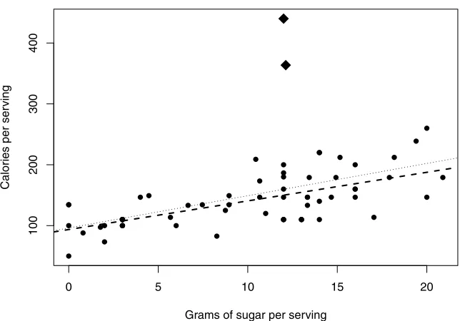
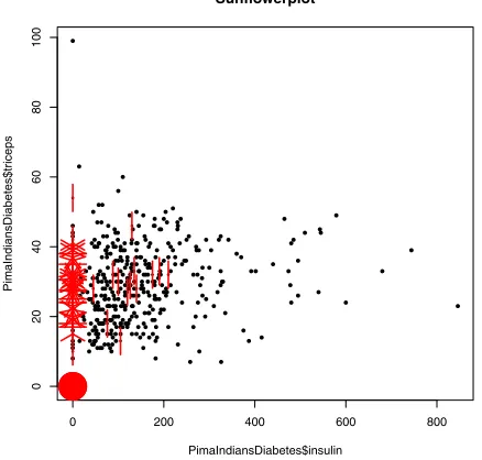
As a specific illustration of this last point, a popular benchmark dataset for evaluating binary classification algorithms (i.e., computational procedures that attempt to predict a binary outcome from other variables) is the Pima Indi-ans diabetes dataset, available from the UCI Machine Learning Repository, an important Internet data source discussed further in Chapter 4. In this partic-ular case, the dataset characterizes female adult members of the Pima Indians tribe, giving a number of different medical status and history characteristics (e.g., diastolic blood pressure, age, and number of times pregnant), along with a binary diagnosis indicator with the value 1 if the patient had been diagnosed with diabetes and 0 if they had not. Several versions of this dataset are avail-able: the one considered here was the UCI website on May 10, 2014, and it has 768 rows and 9 columns. In contrast, the data frame Pima.trincluded inR’s

MASS package is a subset of this original, with 200 rows and 8 columns. The metadata available for this dataset from the UCI Machine Learning Repository now indicates that this dataset exhibits missing values, but there is also a note that prior to February 28, 2011 the metadata indicated that there were no miss-ing values. In fact, the missmiss-ing values in this dataset are not coded explicitly as missing with a special code (e.g., R’s“NA” code), but are instead coded as zero. As a result, a number of studies characterizing binary classifiers have been published using this dataset as a benchmark where the authors were not aware that data values were missing, in some cases, quite a large fraction of the total observations. As a specific example, the serum insulin measurement included in the dataset is 48.7% missing.

(19)

Is Pluto a Planet? [72], astronomer David Weintraub argues that Pluto should remain a planet, based on the following defining criteria for planethood:

1. the object must be too small to generate, or to have ever generated, energy through nuclear fusion;

2. the object must be big enough to be spherical;

3. the object must have a primary orbit around a star.

The first of these conditions excludes dwarf stars from being classed as planets, and the third excludes moons from being declared planets (since they orbit planets, not stars). Weintraub notes, however, that under this definition, there are at least 24 planets orbiting the Sun: the eight now generally regarded as planets, Pluto, and 15 of the largest objects from the asteroid belt between Mars and Jupiter and from the Kuiper Belt beyond Pluto. This example illustrates that definitions are both extremely important and not to be taken for granted: everyone knows what a planet is, don’t they? In the broader context of data analysis, the key point is that unrecognized disagreements in the definition of a variable are possible between those who measure and record it, and those who subsequently use it in analysis; these discrepancies can lie at the heart of unexpected findings that turn out to be erroneous. For example, if we wish to combine two medical datasets, characterizing different groups of patients with “the same” disease, it is important that the same diagnostic criteria be used to declare patients “diseased” or “not diseased.” For a more detailed discussion of the role of definitions in data analysis, refer toSec. 2.4ofExploring Data in Engineering, the Sciences, and Medicine[58]. (Although the book is generally quite mathematical, this is not true of the discussions of data characteristics presented inChapter 2, which may be useful to readers of this book.)

1.2.2 Exploratory analysis

Roughly speaking, exploratory data analysis (EDA) may be defined as the art of looking at one or more datasets in an effort to understand the underlying structure of the data contained there. A useful description of how we might go about this is offered by Diaconis [21]:

We look at numbers or graphs and try to find patterns. We pursue leads suggested by background information, imagination, patterns perceived, and experience with other data analyses.

(20)

can be particularly useful in exploring data when the number of levels—i.e., the number of distinct values the original variable can exhibit—is relatively small. In such cases, many useful exploratory tools have been developed that allow us to examine the character of these nonnumeric variables and their relationship with other variables, whether categorical or numeric. Simple graphical exam-ples include boxplots for looking at the distribution of numerical values across the different levels of a categorical variable, or mosaic plots for looking at the relationship between categorical variables; both of these plots and other, closely related ones are discussed further inChapters 2and3.

Categorical variables with many levels pose more challenging problems, and these come in at least two varieties. One is represented by variables like U.S. postal zipcode, which identifies geographic locations at a much finer-grained level than state does and exhibits about 40,000 distinct levels. A detailed dis-cussion of dealing with this type of categorical variable is beyond the scope of this book, although one possible approach is described briefly at the end of

Chapter 10. The second type of many-level categorical variable arises in settings

where the inherent structure of the variable can be exploited to develop special-ized analysis techniques. Text data is a case in point: the number of distinct words in a document or a collection of documents can be enormous, but special techniques for analyzing text data have been developed. Chapter 8 introduces some of the methods available in Rfor analyzing text data.

The mention of “graphs” in the Diaconis quote is particularly important since humans are much better at seeing patterns in graphs than in large collec-tions of numbers. This is one of the reasonsRsupports so many different graph-ical display methods (e.g., scatterplots, barplots, boxplots, quantile-quantile plots, histograms, mosaic plots, and many, many more), and one of the reasons this book places so much emphasis on them. That said, two points are important here. First, graphical techniques that are useful to the data analyst in finding important structure in a dataset are not necessarily useful in explaining those findings to others. For example, large arrays of two-variable scatterplots may be a useful screening tool for finding related variables or anomalous data subsets, but these are extremely poor ways of presenting results to others because they essentially require the viewer to repeat the analysis for themselves. Instead, re-sults should be presented to others using displays that highlight and emphasize the analyst’s findings to make sure that the intended message is received. This distinction between exploratoryandexplanatorydisplays is discussed further in

Chapter 2 on graphics inRand inChapter 6on crafting data stories (i.e.,

ex-plaining your findings), but most of the emphasis in this book is on exploratory graphical tools to help us obtain these results.

(21)

library(MASS)

library(car)

par(mfrow=c(2,2))

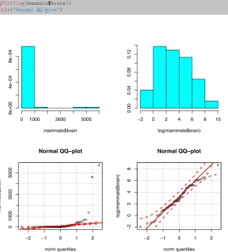
truehist(mammals$brain)

truehist(log(mammals$brain))

qqPlot(mammals$brain)

title("Normal QQ-plot")

qqPlot(log(mammals$brain))

title("Normal QQ-plot")

0 1000 3000 5000

0e+00

4e−04

8e−04

mammals$brain

−2 0 2 4 6 8 10

0.00

0.04

0.08

0.12

log(mammals$brain)

−2 −1 0 1 2

0

1000

3000

5000

norm quantiles

mammals$br

ain

● ● ● ●●●●●●●●●●●●●●●●●●●●●●●●●●●●●●●●●●●●●●●●●●●●●●●●● ●●●●●●●

● ●

●

Normal QQ−plot

−2 −1 0 1 2

−2

0

2

4

6

8

norm quantiles

log(mammals$br

ain)

● ●● ●●

●●● ●●●●

●●●●●●● ●●●●

●●●●●●●● ●●●●

●●●●●● ●●●●●●

●●●● ●●●●●●

●● ●

● ●

Normal QQ−plot

Figure 1.1: Two pairs of characterizations of the brain weight data from the

mammals data frame: histograms and normal QQ-plots constructed from the raw data (left-hand plots), and from log-transformed data (right-hand plots).

(22)

here, which are histograms (top two plots) and normal QQ-plots (bottom two plots). In both cases, these plots are attempting to tell us something about the distribution of data values, and the point of this example is that the extent to which these plots are informative depends strongly on how we prepare the data from which they are constructed. Here, the left-hand pair of plots were generated from the raw data values and they are much less informative than the right-hand pair of plots, which were generated from log-transformed data. In particular, these plots suggest that the log-transformed data exhibits a roughly Gaussian distribution, further suggesting that working with the log of brain weight may be more useful than working with the raw data values. This example is revisited and discussed in much more detail inChapter 3, but the point here is that exactly what we plot—e.g., raw data values vs. log-transformed data values—sometimes matters a lot more than how we plot it.

Since it is one of the main themes of this book, a much more extensive in-troduction to exploratory data analysis is given inChapter 3. Three key points to note here are, first, that exploratory data analysis makes extensive use of graphical tools, for the reasons outlined above. Consequently, the wide and growing variety of graphical methods available inRmakes it a particularly suit-able environment for exploratory analysis. Second, exploratory analysis often involves characterizing many different variables and/or data sources, and com-paring these characterizations. This motivates the widespread use of simple and well-known summary statistics like means, medians, and standard deviations, along with other, less well-known characterizations like the MAD scale estimate introduced in Chapter 3. Finally, third, an extremely important aspect of ex-ploratory data analysis is the search for “unusual” or “anomalous” features in a dataset. The notion of anoutlieris introduced briefly inSec. 1.3, but a more detailed discussion of this and other data anomalies is deferred untilChapter 3, where techniques for detecting these anomalies are also discussed.

1.2.3 Computers, software, and R

To useR—or any other data analysis environment—involves three basic tasks:

1. Make the data you want to analyze available to the analysis software;

2. Perform the analysis;

3. Make the results of the analysis available to those who need them.

(23)

briefly addresses the question of “why useRand not something else?” Finally, since this is a book about usingRto analyze data, some key details about the structure of theRlanguage are presented in the third section below.

General structure of a computing environment

In his book,Introduction to Data Technologies[56, pp. 211–214], Paul Murrell describes the general structure of a computing environment in terms of the following six components:

1. theCPUor central processing unitis the basic hardware that does all of the computing;

2. the RAM or random access memory is the internal memory where the CPU stores and retrieves results;

3. thekeyboard is the standard interface that allows the user to submit re-quests to the computer system;

4. thescreenis the graphical display terminal that allows the user to see the results generated by the computer system;

5. themass storage, typically a “hard disk,” is the externalmemory where data and results can be stored permanently;

6. thenetworkis an external connection to the outside world, including the Internet but also possibly anintranetof other computers, along with pe-ripheral devices like printers.

(24)

Closely associated with the CPU is theoperating system, which is the soft-ware that runs the computer system, making useful activity possible. That is, the operating system coordinates the different components, establishing and managing file systems that allow datasets to be stored, located, modified, or deleted; providing user access to programs likeR; providing the support infras-tructure required so these programs can interact with network resources, etc. In addition to the general computing infrastructure provided by the operating system, to analyze data it is necessary to have programs like R and possibly others (e.g., database programs). Further, these programs must be compatible with the operating system: on popular desktops and enterprise servers, this is usually not a problem, although it can become a problem for older operating systems. For example, Section 2.2of the R FAQ document available from the R“Help” tab notes that “support for Mac OS Classic ended with R 1.7.1.”

With the growth of the Internet as a data source, it is becoming increasingly important to be able to retrieve and process data from it. Unfortunately, this involves a number of issues that are well beyond the scope of this book (e.g., parsing HTML to extract data stored in web pages). A brief introduction to the key ideas with some simple examples is given in Chapter 4, but for those needing a more thorough treatment, Murrell’s book is highly recommended [56].

Data analysis software

A key element of the data analysis chain (acquire → analyze → explain) de-scribed earlier is the choice of data analysis software. Since there are a number of possibilities here, why R? One reason is that R is a free, open-source lan-guage, available for most popular operating systems. In contrast, commercially supported packages must be purchased, in some cases for a lot of money.

Another reason to useRin preference to other data analysis platforms is the enormous range of analysis methods supported byR’sgrowing universe of add-on packages. These packages support analysis methods from many branches of statistics (e.g., traditional statistical methods like ANOVA, ordinary least squares regression, and t-tests, Bayesian methods, and robust statistical pro-cedures), machine learning (e.g., random forests, neural networks, and boosted trees), and other applications like text analysis. This availability of methods is important because it greatly expands the range of data exploration and analysis approaches that can be considered. For example, if you wanted to use the mul-tivariate outlier detection method described in Chapter 9 based on the MCD covariance estimator in another framework—e.g., Microsoft Excel—you would have to first build these analysis tools yourself, and then test them thoroughly to make sure they are really doing what you want. All of this takes time and effort just to be able to get to the point of actually analyzing your data.

(25)

2017, was available from the website:

http://spectrum.ieee.org/computing/software/ the-2017-top-ten-programming-languages

The top six programming languages on this list were, in descending order: Python, C, Java, C++, C#, and R. Note that the top five of these are general-purpose languages, all suitable for at least two of the four programming environ-ments considered in the survey: web, mobile, desktop/enterprise, and embed-ded. In contrast,Ris a specialized data analysis language that is only suitable for the desktop/enterprise environment. The next data analysis language in this list was the commercial package MATLABR

, ranked 15th.

The structure of R

TheRprogramming language basically consists of three components:

• a set of base R packages, a required collection of programs that support language infrastructure and basic statistics and data analysis functions;

• a set of recommended packages, automatically included in almost all R installations (theMASS package used in this chapter belongs to this set);

• a very large and growing set ofoptional add-on packages, available through the Comprehensive R Archive Network (CRAN).

MostR installations have all of the base and recommended packages, with at least a few selected add-on packages. The advantage of this language structure is that it allows extensive customization: as of February 3, 2018, there were 12,086 packages available from CRAN, and new ones are added every day. These packages provide support for everything from rough and fuzzy set theory to the analysis of twitter tweets, so it is an extremely rare organization that actually needseverythingCRAN has to offer. Allowing users to install only what they need avoids massive waste of computer resources.

(26)

It is important to note thatinstallinganRpackage makes it available for you to use, but this doesnot“load” the package into your currentRsession. To do this, you must use thelibrary()function, which works in two different ways. First, if you enter this function without any parameters—i.e., type “library()” at theRprompt—it brings up a new window that lists all of the packages that have been installed on your machine. To use any of these packages, it is necessary to use the library() command again, this time specifying the name of the package you want to use as a parameter. This is shown in the code appearing at the top ofFig. 1.1, where theMASSandcarpackages are loaded:

library(MASS)

library(car)

The first of these commands loads theMASSpackage, which contains themammals

data frame and the truehistfunction to generate histograms, and the second loads thecarpackage, which contains theqqPlotfunction used to generate the normal QQ-plots shown in Fig. 1.1.

1.3 A representative R session

To give a clear view of the essential material covered in this book, the following paragraphs describe a simple but representative R analysis session, providing a few specific illustrations of what R can do. The general task is a typical preliminary data exploration: we are given an unfamiliar dataset and we begin by attempting to understand what is in it. In this particular case, the dataset is a built-in data example from R—one of many such examples included in the language—but the preliminary questions explored here are analogous to those we would ask in characterizing a dataset obtained from the Internet, from a data warehouse of customer data in a business application, or from a computerized data collection system in a scientific experiment or an industrial process monitoring application. Useful preliminary questions include:

1. How many records does this dataset contain?

2. How many fields (i.e., variables) are included in each record?

3. What kinds of variables are these? (e.g., real numbers, integers, categorical variables like “city” or “type,” or something else?)

4. Are these variables always observed? (i.e., is missing data an issue? If so, how are missing values represented?)

5. Are the variables included in the dataset the ones we were expecting?

6. Are the values of these variables consistent with what we expect?

(27)

The example presented here does not address all of these questions, but it does consider some of them and it shows how theRprogramming environment can be useful in both answering and refining these questions.

AssumingRhas been installed on your machine (if not, see the discussion of installingRin Chapter 11), you begin an interactive session by clicking on the Ricon. This brings up a window where you enter commands at the “>” prompt to tellRwhat you want to do. There is a toolbar at the top of this display with a number of tabs, including “Help” which provides links to a number of useful documents that will be discussed further in later parts of this book. Also, when you want to end yourRsession, type the command “q()” at the “>” prompt: this is the “quit” command, which terminates your R session. Note that the parentheses after “q” are important here: this tells R that you are calling a function that, in general, does something to the argument or arguments you pass it. In this case, the command takes no arguments, but failing to include the parentheses will causeRto search for an object (e.g., a vector or data frame) named “q” and, if it fails to find this, display an error message. Also, note that when you end yourRsession, you will be asked whether you want to save your workspace image: if you answer “yes,”Rwill save a copy of all of the commands you used in your interactive session in the file.Rhistoryin the current working directory, making this command history—but not the Robjects created from these commands—available for your nextRsession.

Also, in contrast to some other languages—SASR

is a specific example—it is important to recognize thatRis case-sensitive: commands and variables in lower-case, upper-case, or mixed-case arenotthe same inR. Thus, while aSAS procedure likePROC FREQ may be equivalently invoked as proc freqor Proc Freq, theRcommandsqqplotandqqPlotarenotthe same: qqplotis a func-tion in thestatspackage that generates quantile-quantile plots comparing two empirical distributions, whileqqPlotis a function in thecarpackage that gen-erates quantile-quantile plots comparing a data distribution with a theoretical reference distribution. While the tasks performed by these two functions are closely related, the details of what they generate are different, as are the details of their syntax. As a more immediate illustration ofR’scase-sensitivity, recall that the functionq() “quits” yourR session; in contrast, unless you define it yourself or load an optional package that defines it, the functionQ()does not exist, and invoking it will generate an error message, something like this:

Q()

## Error in Q(): could not find function "Q"

(28)

Mr Derek Whiteside of the UK Building Research Station recorded the weekly gas consumption and average external temperature at his own house in south-east England for two heating seasons, one of 26 weeks before, and one of 30 weeks after cavity-wall insulation was installed. The object of the exercise was to assess the effect of the insulation on gas consumption.

To analyze this dataset, it is necessary to first make it available by loading the

MASS package with thelibrary()function as described above:

library(MASS)

An R data frame is a rectangular array of N records—each represented as a row—withM fields per record, each representing a value of a particular variable for that record. This structure may be seen by applying the head function to thewhitesidedata frame, which displays its first few records:

head(whiteside)

## Insul Temp Gas ## 1 Before -0.8 7.2 ## 2 Before -0.7 6.9 ## 3 Before 0.4 6.4 ## 4 Before 2.5 6.0 ## 5 Before 2.9 5.8 ## 6 Before 3.2 5.8

More specifically, the first line lists the field names, while the next six lines show the values recorded in these fields for the first six records of the dataset. Re-call from the discussion above that thewhitesidedata frame characterizes the weekly average heating gas consumption and the weekly average outside temper-ature for two successive winters, the first before Whiteside installed insulation in his house, and the second after. Thus, each record in this data frame rep-resents one weekly observation, listing whether it was made before or after the insulation was installed (the Insulvariable), the average outside temperature, and the average heating gas consumption.

A more detailed view of this data frame is provided by the str function, which returns structural characterizations of essentially anyRobject. Applied to thewhitesidedata frame, it returns the following information:

str(whiteside)

## 'data.frame': 56 obs. of 3 variables:

## $ Insul: Factor w/ 2 levels "Before","After": 1 1 1 1 1 1 1 1 1 1 ... ## $ Temp : num -0.8 -0.7 0.4 2.5 2.9 3.2 3.6 3.9 4.2 4.3 ...

## $ Gas : num 7.2 6.9 6.4 6 5.8 5.8 5.6 4.7 5.8 5.2 ...

Here, the first line tells us thatwhitesideis a data frame, with 56 observations (rows or records) and 3 variables. The second line tells us that the first variable,

(29)

an importantRdata type used to represent categorical data, introduced briefly in the next paragraph.) The third and fourth lines tell us thatTempandGasare numeric variables. Further, all lines except the first provide summaries of the first few (here, 10) values observed for each variable. For the numeric variables, these values are the same as those shown with the head command presented above, while for factors,strdisplays a numerical index indicating which of the possible levels of the variable is represented in each of the first 10 records.

Because factor variables are both very useful and somewhat more complex in their representation than numeric variables, it is worth a brief digression here to say a bit more about them. Essentially, factor variables inRare special vectors used to represent categorical variables, encoding them with two components: a level, corresponding to the value we see (e.g., “Before” and “After” for the factor

Insulin the whitesidedata frame), and an index that maps each element of the vector into the appropriate level:

x <- whiteside$Insul

str(x)

## Factor w/ 2 levels "Before","After": 1 1 1 1 1 1 1 1 1 1 ...

x[2]

## [1] Before

## Levels: Before After

Here, thestrcharacterization tells us how many levels the factor has and what the names of those levels are (i.e., two levels, named “Before” and “After”), but the values strdisplays are the indices instead of the levels (i.e., the first 10 records list the the first value, which is “Before”). R also supports charac-ter vectors and these could be used to represent categorical variables, but an important difference is that the levels defined for a factor variable represent its only possible values: attempting to introduce a new value into a factor variable fails, generating a missing value instead, with a warning. For example, if we attempted to change the second element of this factor variable from “Before” to “Unknown,” we would get a warning about an invalid factor level and that the attempted assignment resulted in this element having the missing valueNA. In contrast, if we convertxin this example to a character vector, the new value assignment attempted above now works:

x <- as.character(whiteside$Insul)

str(x)

## chr [1:56] "Before" "Before" "Before" "Before" "Before" "Before" ...

x[2]

## [1] "Before"

x[2] <- "Unknown" str(x)

(30)

In addition tostrandhead, thesummaryfunction can also provide much useful information about data frames and other R objects. In fact, summary is an example of a generic function inR, that can do different things depending on the attributes of the object we apply it to. Generic functions are discussed further inChapters 2and7, but when the genericsummaryfunction is applied to a data frame like whiteside, it returns a relatively simple characterization of the values each variable can assume:

summary(whiteside)

## Insul Temp Gas

## Before:26 Min. :-0.800 Min. :1.300 ## After :30 1st Qu.: 3.050 1st Qu.:3.500

## Median : 4.900 Median :3.950

## Mean : 4.875 Mean :4.071

## 3rd Qu.: 7.125 3rd Qu.:4.625

## Max. :10.200 Max. :7.200

This result may be viewed as a table with one column for each variable in thewhitesidedata frame—Insul,Temp, andGas—with a column format that depends on the type of variable being characterized. For the two-level factor

Insul, the summary result gives the number of times each possible level oc-curs: 26 records list the value “Before,” while 30 list the value “After.” For the numeric variables, the result consists of two components: one is the mean value—i.e., the average of the variable over all records in the dataset—while the other isTukey’s five-number summary, consisting of these five numbers:

1. thesample minimum, defined as the smallest value ofxin the dataset;

2. the lower quartile, defined as the value xL for which 25% of the data satisfiesx≤xL and the other 75% of the data satisfiesx > xL;

3. thesample median, defined as the “middle value” in the dataset, the value that 50% of the data values do not exceed and 50% do exceed;

4. the upper quartile, defined as the value xU for which 75% of the data satisfiesx≤xU and the other 25% of the data satisfiesx > xU;

5. thesample maximum, defined as the largest value ofxin the dataset.

(31)

●

Before After

2

3

4

5

6

7

Figure 1.2: Side-by-side boxplot comparison of the “Before” and “After” subsets of theGasvalues from thewhitesidedata frame.

An extremely useful graphical representation of Tukey’s five-number sum-mary is the boxplot, particularly useful in showing how the distribution of a numerical variable depends on subsets defined by the different levels of a factor.

Fig. 1.2 shows a side-by-side boxplot summary of theGasvariable for subsets

of thewhitesidedata frame defined by theInsulvariable. This summary was generated by the followingRcommand, which uses theR formula interface(i.e.,

Gas ~ Insul) to request boxplots of the ranges of variation of theGasvariable for each distinct level of theInsulfactor:

boxplot(Gas ~ Insul, data = whiteside)

(32)

Insul

Figure 1.3: The 3×3 plot array generated by plot(whiteside).

bottom horizontal line does not represent the sample minimum, but the “small-est non-outlying value” where the determination of what values are “outlying” versus “non-outlying” is made using a simple rule discussed inChapter 3.

Fig. 1.3 shows the results of applying theplot function to thewhiteside

(33)

● ● ●

● ●●

●● ● ●

● ● ● ●● ●

● ● ● ● ●●

● ●

● ●●

● ●● ●● ●

● ● ● ●● ●

● ●● ● ● ● ●

● ● ●

● ●

● ● ●

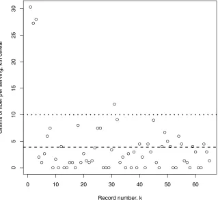
0 10 20 30 40 50

0

2

4

6

8

10

Index

whiteside$T

emp

Figure 1.4: The result of plot(whiteside$Temp).

In Fig. 1.4, applying plot to the Temp variable from the whiteside data

frame shows howTemp varies with its record number in the data frame. Here, these values appear in two groups—one of 26 points, followed by another of 30 points—but within each group, they appear in ascending order. From the data description presented earlier, we might expect these values to represent average weekly winter temperatures recorded in successive weeks during the two heating seasons characterized in the dataset. Instead, these observations have been ordered from coldest to warmest within each heating season. While such unexpected structure often makes no difference, it sometimes does; the key point here is that plotting the data can reveal it.

Fig. 1.5shows the result of applying theplotfunction to the factor variable

(34)

Before After

0

5

10

15

20

25

30

Figure 1.5: The result of plot(whiteside$Insul).

The rest of this section considers some refinements of the scatterplot between weekly average heating gas consumption and average outside temperature ap-pearing in the three-by-three plot array in Fig. 1.3. The intent is to give a “preview of coming attractions,” illustrating some of the ideas and techniques that will be discussed in detail in subsequent chapters.

The first of these extensions is Fig. 1.6, which plotsGas versus Temp with different symbols for the two heating seasons (i.e., “Before” and “After”). The followingRcode generates this plot, using open triangles for the “Before” data and solid circles for the “After” data:

plot(whiteside$Temp, whiteside$Gas, pch=c(6,16)[whiteside$Insul])

(35)

●

●●

● ●● _●

● ●

● ● ●●

● ●

● ● ●

●●

● ●

● ● ●

●

● ●

0 2 4 6 8 10

2

3

4

5

6

7

whiteside$Temp

whiteside$Gas

Figure 1.6: Scatterplot ofGasversusTempfrom thewhitesidedata frame, with distinct point shapes for the “Before” and “After” data subsets.

Fig. 1.7 shows a simple but extremely useful modification of Fig. 1.6: the

inclusion of a legend that tells us what the different point shapes mean. This is also quite easy to do, using thelegendfunction, which can be used to put a box anywhere we like on the plot, displaying the point shapes we used together with descriptive text to tell us what each shape means. TheRcode used to add this legend is shown inFig. 1.7.

The last example considered here adds tworeference linesto the plot shown

inFig. 1.7. These lines are generated using theRfunctionlm, which fitslinear

regression models, discussed in detail inChapter 5. These models represent the simplest type ofpredictive model, a topic discussed more generally in Chapter 10where other classes of predictive models are introduced. The basic idea is to construct a mathematical model that predicts a response variable from one or more other, related variables. In the whiteside data example considered here, these models predict the weekly average heating gas consumed as a linear function of the measured outside temperature. To obtain two reference lines, one model is fit for each of the data subsets defined by the two values of the

Insul variable. Alternatively, we could obtain the same results by fitting a single linear regression model to the dataset, using both theTemp and Insul

variables as predictors. This alternative approach is illustrated in Chapter 5

(36)

legend(x="topright",legend=c("Insul = Before","Insul = After"), pch=c(6,16))

●

●●

● ●●

●_●

● ●

● ● ● ●●

● ●_●

● ●

●●

● ●

● ● ●

●

● ●

0 2 4 6 8 10

2

3

4

5

6

7

whiteside$Temp

whiteside$Gas

●

Insul = Before Insul = After

Figure 1.7: Scatterplot from Fig. 1.6with a legend added to identify the two data subsets represented with different point shapes.

Fig. 1.8 is the same as Fig. 1.7, but with these reference lines added. As

with the different plotting points, these lines are drawn with different line types. The R code listed at the top of Fig. 1.8 first re-generates the previous plot, then fits the two regression models just described, and finally draws in the lines determined by these two models. Specifically, the dashed “Before” line is obtained by fitting one model to only the “Before” points and the solid “After” line is obtained by fitting a second model to only the “After” points.

1.4 Organization of this book

(37)

legend(x="topright",legend=c("Insul = Before","Insul = After"), pch=c(6,16)) Model1 <- lm(Gas ~ Temp, data = whiteside, subset = which(Insul == "Before")) Model2 <- lm(Gas ~ Temp, data = whiteside, subset = which(Insul == "After"))

abline(Model1, lty=2)

abline(Model2)

●

●●

● ●●

● ● ●

● ●

● ● ●●

● ●

● ● ●

●●

● ●

● ● ●

●

● ●

0 2 4 6 8 10

2

3

4

5

6

7

whiteside$Temp

whiteside$Gas

●

Insul = Before Insul = After

Figure 1.8: Scatterplot fromFig. 1.7with linear regression lines added, repre-senting the relationships betweenGasandTempfor each data subset.

More specifically, the first part of this book consists of the first seven chap-ters, including this one. As noted, one of the great strengths ofRis its variety of powerful data visualization procedures, andChapter 2provides a detailed intro-duction to several of these. This subject is introduced first because it provides those with little or no priorRexperience a particularly useful set of tools that they can use right away. Specific topics include both basic plotting tools and some simple customizations that can make these plots much more effective. In fact,R supports several different graphics environments which, unfortunately, don’t all play well together. The most important distinction is that between base graphics—the primary focus ofChapter 2—and the alternativegrid graph-icssystem, offering greater flexibility at the expense of being somewhat harder to use. While base graphics are used for most of the plots in this book, a number of important Rpackages use grid graphics, including the increasingly popular

(38)

fail if we attempt to use base graphics constructs with plots generated by an Rpackage based on grid graphics. For this reason, it is important to be aware of the different graphics systems available inR, even if we work primarily with base graphics as we do in this book. SinceRsupports color graphics, two sets of color figures are included in this book, the first collected as Chapter 2.8and the second collected asChapter 9.10in the second part of the book.

Chapter 3introduces the basic notions of exploratory data analysis (EDA),

focusing on specific techniques and their implementation in R. Topics include descriptive statistics like the mean and standard deviation, essential graphical tools like scatterplots and histograms, an overview of data anomalies (including brief discussions of different types, why they are too important to ignore, and a few of the things we can do about them), techniques for assessing or visualizing relationships between variables, and some simple summaries that are useful in characterizing large datasets. This chapter is one of two devoted to EDA, the second beingChapter 9in the second part of the book, which introduces some more advanced concepts and techniques.

The introductoryRsession example presented in Sec. 1.3was based on the

whitesidedata frame, an internalRdataset included in theMASSpackage. One of the great conveniences in learning R is the fact that so many datasets are available as built-in data objects. Conversely, for R to be useful in real-world applications, it is obviously necessary to be able to bring the data we want to analyze into our interactiveRsession. This can be done in a number of different ways, and the focus ofChapter 4is on the features available for bringing external data into ourRsession and writing it out to be available for other applications. This latter capability is crucial since, as emphasized in Sec. 1.2.3, everything within our active R session exists in RAM, which is volatile and disappears forever when we exit this session; to preserve our work, we need to save it to a file. Specific topics discussed in Chapter 4include data file types, some ofR’s commands for managing external files (e.g., finding them, moving them, copying or deleting them), some of the built-in procedures R provides to help us find and import data from the Internet, and a brief introduction to the important topic ofdatabases, the primary tool for storing and managing data in businesses and other large organizations.

Chapter 5 is the first of two chapters introducing the subject of predictive

(39)

practical problems can be re-cast into exactly this form,Chapter 5begins with a detailed treatment of this problem. From there, more generallinear regression problems are discussed in detail, including the problem ofoverfittingand how to protect ourselves from it, the use of multiple predictors, the incorporation of categorical variables, how to include interactions and transformations in a linear regression model, and a brief introduction to robust techniques that are resistant to the potentially damaging effects of outliers.

When we analyze data, we are typically attempting to understand or predict something that is of interest to others, which means we need to show them what we have found. Chapter 6is concerned with the art of craftingdata stories to meet this need. Two key details are, first, that different audiences have different needs, and second, that most audiences want a summary of what we have done and found, and not a complete account with all details, including wrong turns and loose ends. The chapter concludes with three examples of moderate-length data stories that summarize what was analyzed and why, and what was found without going into all of the gory details of how we got there (some of these details are important for the readers of this book even if they don’t belong in the data story; these details are covered in other chapters).

The second part of this book consists of Chapters 7 through11, introduc-ing the topics of R programming, the analysis of text data, second looks at exploratory data analysis and predictive modeling, and the challenges of orga-nizing our work. Specifically,Chapter 7introduces the topic of writing programs inR. Readers with programming experience in other languages may want to skip or skim the first part of this chapter, but theR-specific details should be useful to anyone without a lot of prior R programming experience. As noted in the Preface, this book assumes no prior programming experience, so this chapter starts simply and proceeds slowly. It begins with the question of why we should learn to program inRrather than just rely on canned procedures, and contin-ues through essential details of both the structure of the language (e.g., data types like vectors, data frames, and lists; control structures like for loops and if statements; and functions in R), and the mechanics of developing programs (e.g., editing programs, the importance of comments, and the art of debugging). The chapter concludes with five programming examples, worked out in detail, based on the recognition that many of us learn much by studying and modifying code examples that are known to work.

(40)

to which various types of quantitative analysis procedures may then be applied. Many of the techniques required to do this type of analysis are provided by the R packages tm and quanteda, which are introduced and demonstrated in the discussion presented here. Another key issue in analyzing text data is the impor-tance ofpreprocessingto address issues like inconsistencies in capitalization and punctuation, and the removal of numbers, special symbols, and non-informative stopwordslike “a” or “the.” Text analysis packages liketmandquantedainclude functions to perform these operations, but many of them can also be handled using low-level string handling functions like grep, gsub, and strsplit that are available in baseR. Both because these functions are often extremely useful adjuncts to specialized text analysis packages and because they represent an easy way of introducing some important text analysis concepts, these functions are also treated in some detail inChapter 8. Also, these functions—along with a number of others in R—are based on regular expressions, which can be ex-tremely useful but also exex-tremely confusing to those who have not seen them before;Chapter 8includes an introduction to regular expressions.

Chapter 9provides a second look at exploratory data analysis, building on

the ideas presented in Chapter 3 and providing more detailed discussions of some of the topics introduced there. For example, Chapter 3 introduces the idea of using random variables and probability distributions to model under-tainty in data, along with some standard random variable characterizations like the mean and standard deviation. The basis for this discussion is the popular Gaussian distribution, but this distribution is only one of many and it is not always appropriate. Chapter 9 introduces some alternatives, with examples to show why they are sometimes necessary in practice. Other topics introduced in

Chapter 9 include confidence intervals and statistical significance, association

measures that summarize the relationship between variables of different types, multivariate outliers and their impact on standard association measures, and a number of useful graphical tools that build on these ideas. Since color greatly enhances the utility of some of these tools, the second group of color figures follows, as Chapter 9.10.

Following this second look at exploratory data analysis,Chapter 10builds on the discussion of linear regression models presented in Chapter 5, introducing a range of extensions, including logistic regression for binary responses (e.g., the Moneyballproblem: estimate the probability of having a successful major league career, given college baseball statistics), more general approaches to these binary classification problems like decision trees, and a gentle introduction to the increasingly popular arena of machine learning models like random forests and boosted trees. Because predictive modeling is a vast subject, the treatment presented here is by no means complete, but Chapters 5and10should provide a useful introduction and serve as a practical starting point for those wishing to learn more.