This book prepares readers to analyze data and interpret statistical results usingRmore quickly than other texts. R is a challenging program to learn because code must be created to get started. To alleviate that challenge, Professor Gerbing developedlessR. The extensions provided
by lessR remove the need to program. By introducing R through lessR, readers learn how
to organize data for analysis, read the data into R, and produce output without performing numerous functions and programming exercises first. With lessR, readers can select the necessary procedure and change the relevant variables without programming. The text reviews basic statistical procedures with thelessRenhancements added to the standardRenvironment, complete with input, output, and an extensive interpretation of the results. Through the use of
lessR,Rbecomes immediately accessible to the novice user and easier to use for the experienced user.
Highlights of the book include:
• Quick startsthat introduce readers to the concepts and commands reviewed in the chapters. • Margin notes that highlight, define, illustrate, and cross-reference the key concepts. When readers encounter a term previously discussed, the margin notes identify the page number to the initial introduction.
• Scenariosthat highlight the use of a specific analysis followed by the correspondingR/lessR
input and an interpretation of the resulting output.
• Numerous examples of outputfrom psychology, business, education, and other social sciences, that demonstrate how to interpret results.
• Two data sets, provided on the book’s website and analyzed multiple times in the book, provide continuity throughout.
• End of chapter worked problemshelp readers test their understanding of the concepts.
• A website at www.lessRstats.com that features the lessR program, the book’s data sets referenced in standard text and SPSS formats so readers can practice using R/lessR by working through the text examples and worked problems, PDF slides for each chapter, solutions to the book’s worked problems, links to R/lessR videos to help readers better understand the program, and more.
An ideal supplement for graduate or advanced undergraduate courses in statistics, research methods, or any course in which R is used, taught in departments of psychology, business, education, and other social and health sciences, this book will also be appreciated by researchers interested in using R for their data analysis. Prerequisites include basic statistical knowledge. Knowledge ofR is not assumed.
PROGRAMMING
711 Third Avenue, New York, NY 10017 and by Routledge
27 Church Road, Hove, East Sussex BN3 2FA
Routledge is an imprint of the Taylor & Francis Group, an informa business © 2014 Taylor & Francis
The right of David W. Gerbing to be identified as author of this work has been asserted by him in accordance with sections 77 and 78 of the Copyright, Designs and Patents Act 1988.
All rights reserved. No part of this book may be reprinted or reproduced or utilised in any form or by any electronic, mechanical, or other means, now known or hereafter invented, including photocopying and recording, or in any information storage or retrieval system, without permission in writing from the publishers.
Trademark notice:Product or corporate names may be trademarks or registered trademarks, and are used only for identification and explanation without intent to infringe.
Library of Congress Cataloging in Publication Data Gerbing, David W.
R data analysis without programming / David Gerbing. pages cm
1. R (Computer program language) 2. Mathematical statistics–Data processing. I. Title.
QA276.45.R3G46 2013
519.50285’5133–dc23 2013024185
ISBN: 978-0-415-64173-9 (hbk) ISBN: 978-0-415-65720-4 (pbk) ISBN: 978-1-315-85675-9 (ebk)
Rachel Maculan Sodré
Preface xiii
About the Author xvii
CHAPTER 1 Rfor Data Analysis 1
CHAPTER 2 Read/Write Data 31
CHAPTER 3 Edit Data 53
CHAPTER 4 Categorical Variables 77
CHAPTER 5 Continuous Variables 99
CHAPTER 6 Means, Compare Two Samples 123
CHAPTER 7 Compare Multiple Samples 149
CHAPTER 8 Correlation 181
CHAPTER 9 Regression I 203
CHAPTER 10 Regression II 223
CHAPTER 11 Factor/Item Analysis 251
Appendix: StandardRCode 279
Notes 283
References 285
Preface xiii
About the Author xvii
CHAPTER 1
R
for Data Analysis
1
1.1 Introduction 1
1.2 Access R 3
1.3 UseR 6
1.4 RGraphs 16
1.5 Reproducible Code 19
1.6 Data 20
Worked Problems 28
CHAPTER 2
Read/Write Data
31
2.1 Quick Start 31
2.2 Read Data 32
2.3 More Data Formats 40
2.4 Variable Labels 45
2.5 Write Data 48
Worked Problems 50
CHAPTER 3
Edit Data
53
3.1 Quick Start 53
3.2 Edit Data 54
3.3 Transform Data 55
3.4 Recode Data 62
3.5 Sort Data 66
3.7 Merge Data 72
Worked Problems 75
CHAPTER 4
Categorical Variables
77
4.1 Quick Start 77
4.2 One Categorical Variable 79
4.3 Two Categorical Variables 87
4.4 Onward to the Third Dimension 93
Worked Problems 98
CHAPTER 5
Continuous Variables
99
5.1 Quick Start 99
5.2 Histogram 100
5.3 Summary Statistics 105
5.4 Scatter Plot and Box Plot 110
5.5 Density Plot 114
5.6 Time Plot 118
Worked Problems 121
CHAPTER 6
Means, Compare Two Samples
123
6.1 Quick Start 123
6.2 Evaluate a Single Group Mean 124
6.3 Compare Two Different Groups 130
6.4 Compare Dependent Samples 142
Worked Problems 147
CHAPTER 7
Compare Multiple Samples
149
7.1 Quick Start 149
7.2 One-way ANOVA 150
7.3 Randomized Block ANOVA 158
7.4 Two-way ANOVA 166
7.5 More Advanced Designs 173
Worked Problems 180
CHAPTER 8
Correlation
181
8.1 Quick Start 181
8.2 Relation of Two Numeric Variables 181
8.3 The Correlation Matrix 194
8.4 Non-parametric Correlation Coefficients 200
CHAPTER 9
Regression I
203
9.1 Quick Start 203
9.2 The Regression Model 204
9.3 Residuals and Model Fit 209
9.4 Prediction Intervals 212
9.5 Outliers and Diagnostics 216
Worked Problems 221
CHAPTER 10
Regression II
223
10.1 Quick Start 223
10.2 The Multiple Regression Model 224
10.3 Indicator Variables 234
10.4 Logistic Regression 239
Worked Problems 248
CHAPTER 11
Factor/Item Analysis
251
11.1 Quick Start 251
11.2 Overview of Factor Analysis 252
11.3 Exploratory Factor Analysis 254
11.4 The Scale Score 260
11.5 Confirmatory Factor Analysis 263
11.6 Beyond the Basics 275
Worked Problems 276
Appendix: StandardRCode 279
Notes 283
References 285
Purpose
This book is addressed to the student, researcher, and/or data analyst who wishes to analyze data usingRto answer questions of interest. The structuring of the data for analysis, doing the analysis with the computer, and then interpreting the results are the skills to which this book is directed. Explicit instructions to use the computer for the analysis are provided, but using the computer is the easy part of data analysis, especially with the computer instructions provided in this book. By far, more content of this book is oriented toward the meaning of the analyses and interpretation of the results.
The computational tools discussed in this book are based on the open source and free R system that is becoming the world’s standard for data analysis. Unlike commercial packages, R costs no money and can be installed at will on any Windows, Macintosh or Linux system. By itself, however, R presents a rather steep learning curve as it requires the ability to write computer code to do data analysis. To make data analysis with R more accessible, this book features a set of extensions toR calledlessR. These extensions ease the transition of the new user into using R for data analysis and for many users contain the only computational tools they will need.
The ultimate goal of this book is to makeRaccessible to users ofSPSSand similar commercial packages, and, indeed, help facilitate R to become the preferred choice of any data analysis system. For data analysts with a proclivity for program computer code,Rhas already emerged as the preferred choice. ThelessRextensions toRremove the need to program and so are designed to provide access to Rfor all data analysts. To the extent that R becomes as straightforward to use and as comprehensive in its range of analyses as its commercial alternatives, then it becomes a viable choice as the preferred data analysis system both in the field and for instruction.
This is the first book that follows the format of the manySPSSbased data analysis texts, with emphasis on both the instructions to produce the analysis, plus detailed interpretation of the resulting output. This book, however, applies the R/lessR system for conducting the analysis, made possible with the lessR extensions. Traditional R books on data analysis provide some interpretation, but much more space is required to explain the programming needed to obtain the output.
Intended Audience
of psychology, business, education, and other social and health sciences. The book will also be helpful to researchers interested in using R for their data analysis. Prerequisites include basic statistical knowledge. Knowledge of Ris not assumed.
Overview of Content
The first chapter shows how to download Rand thenlessR from the worldwide network ofR servers, provides an example of data analysis, shows how data are structured for analysis, and discusses general issues for the use of RandlessR.Chapter 2shows how to read the data from a computer file intoR. Then the data often must be modified before analysis begins, the topic ofChapter 3. This editing can include changing individual data values, assigning missing data codes, transforming, recoding, and sorting the data values for a variable, and also sub-setting and merging data tables.
Chapters 4and5show how to obtain the most basic of all data analyses, the counting of how often each data value or groups of similar data values occurred. Chapter 4explains bar charts and related techniques for counting the values of a categorical variable, one with non-numeric data values. Also included are the analysis of two or more variables in the form of bar charts for two variables, mosaic plots for more than two variables and the associated cross-tabulation tables.Chapter 5does the same for numeric variables, which include the histogram and related analyses, the scatter plot for one variable, the box plot, the density plot and the time plot, plus the associated summary statistics.
Chapter 6explains the analysis of the mean of a single sample or of a mean difference across two different samples. Theses analyses are based on the t-test of the mean, the independent-samples t-test and the dependent-samples t-test. The non-parametric alternatives are also provided. Chapter 7 extends the material in Chapter 6 to comparison of many groups with the analysis of variance. The primary designs considered are the one-way independent groups, randomized blocks and two-way independent groups. Also illustrated are the randomized block factorial design and the split-plot factorial. Effect sizes are an integral part of each discussion.
Chapters 8,9, and10focus on correlation and regression analysis.Chapter 8introduces the scatter plot and the correlation coefficient to describe the relation between two variables. Both the usual parametric version and some non-parametric correlation coefficients are presented, as well as the correlation matrix. The subject of Chapter 9is regression analysis of a linear model of a response variable with a single predictor variable. The discussion includes estimation of the model, a consideration of the evaluation of fit, outliers and influential observations, and prediction intervals. Chapter 10 extends this discussion to multiple regression, the analysis of models with multiple predictor variables, and also to logistic regression, the modeling of a response variable that has only two values.
Distinctive Features
Every chapter after thefirst chapterbegins with a brief Quick Start section. The function calls that provide the analyses described in the remainder of the chapter are listed and briefly described. The goal is that the user can immediately invoke the specified analyses and then, as needed, refer to the remainder of the chapter to obtain the details. Each Quick Start section also serves as a convenient summary of the data analysis functions described in that chapter.
This book makes extensive use of margin notes to highlight the concepts discussed within the main text. Each definition is placed in a margin note. The margin notes also provide a concordance, a cross-reference to where in the book a specific concept is first explained and illustrated. When the reader encounters a term previously discussed, the relevant section and page number appear in the margin notes.
The motivation for a specific analysis is presented in what is called a Scenario, highlighted by light gray rules. Following each Scenario is the R/lessR input for a specific analysis, also highlighted by light gray rules. The resulting output is then interpreted. A Listing is a literal copy of computer output, of which there are many throughout this book.
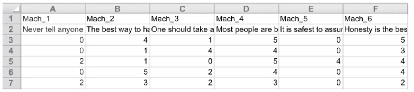
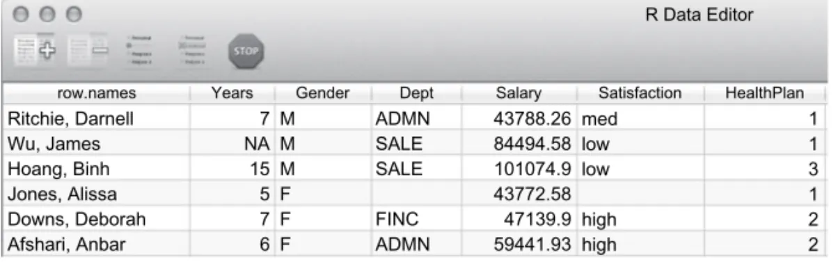
The analysis of many data sets illustrates the concepts discussed in the book. Two data sets, however, are analyzed multiple times to provide continuity throughout. One data set contains some of the typical information found in an employee database, such as each employee’s Gender, Salary and so forth. The other data set regards the measurement of the attitudinal components of Machiavellianism, the tendency to manipulate others for one’s own perceived personal gain. This data set is from a published study by the author in theJournal of Personality and Social Psychology. This study was one of the first applications of confirmatory factor analysis in the psychological literature, and here the analysis is detailed and illustrated to explain both exploratory and confirmatory factor analysis as an integrated strategy for scale development.
lessR
Website
The website to support this book and thelessRpackage is www.lessRstats.com. The site includes a variety of reference materials to support your learning of data analysis, such as the data sets referenced in this book in both standard text andSPSSformats. This way you can practice using
RandlessR, as you read this book and work through the examples and the included worked
problems. Also included are videos on the use of R and lessR, a slide set for each chapter, and solutions, some of which are available only for instructors. The website also provides the opportunity to give your own suggestions and feedback with a place to request upgrades, a place to report bugs, and an interactive forum for asking and getting answers to questions.
Personal Acknowledgments
I would like to acknowledge the helpful people at Routledge/Taylor & Francis who have made this work possible. My editor Debra Riegert expressed an interest in this project from the start and has encouraged and guided the development of this book from its initial conceptualization. Miren Alberro managed the production process with good cheer and the helpful and needed assistance to turn a manuscript into a book.
at Routledge/Taylor & Francis, Jason introduced me to Debra, the introduction from which this book developed. Jason also provided two different forums for presenting my work onlessRat Portland State University: his informal seminars on quantitative topics for faculty and graduate students, and his annual June workshops on quantitative topics.
My students at Portland State University also deserve recognition for their role in the development of lessR and this book. In 2008 some of my students who used Macintosh computers asked me what software they could use for class assignments. I had primarily been using Excel, but at that time Microsoft deleted much of the statistical functionality from the Macintosh version of Excel. My answer was R, but the first classroom experiences withR were not satisfying. Students were frustrated because of all the programming work needed to get anything useful done, and spent more time learning how to use the computer than actually thinking about the meaning of the results – hence lessR and four years of undergraduate and graduate students who have used and contributed much feedback to the project from the beginning of its development through the current version.
R
FOR DATA ANALYSIS
1.1
Introduction
1.1.1 Data Analysis
We ask many questions to which we seek answers. Some of these questions involve the way things work in our world, including our social processes and relationships, and our psychological selves. This book describes analyses based on observations that facilitate answering these types of questions. On average, do men make more than women managers at a particular company? Which of two pain medications is more effective? What College GPA do we forecast for an applicant who has a SAT score of 1130 and a High School GPA of 3.8? Do people generally have trust in others?
To answer questions such as these we seekempiricalanswers. We seek answers based on our
empirical: Information based on observations acquired from our five senses. observations of the world around us: What we see, hear, touch, taste, and smell, in particular,
the measurements of what we observe. Our concern in this book is with observations in the data:
Measurements of different people or whatever the unit of analysis. form ofdata, the varying measurements of different people, organizations, places, things, and
events.
Different measurements generally vary. For example, two different people have different heights, place differing amounts of trust in others, have different blood pressures, and earn different salaries. Height and blood pressure are two of the many variables that can be measured for anyone. For college students, College GPA and incoming High School GPA, and SAT score
are measured variables. data analysis:
Application of statistical methods to transform data into usable information. Data analysis is the application of statistical concepts and methods to transform data,
sometimes vast amounts of data, into usable information. This information is then used to form a conclusion regarding the people or organizations or places or whatever is the topic of interest. In the modern world data analysis is done exclusively on the computer. This book is about doing data analysis with one such computer software system,R, enhanced with lessR.
1.1.2
R
with
lessR
with expensive, proprietary statistical applications. Originally they ran only on IBM mainframe computers, but eventually migrated to PCs as the technology developed.
The cost and exclusivity of competent statistical applications for data analysis is becoming less relevant as the capability and popularity of the R system continues to grow. In terms of pure statistical power to analyze data,R compares favorably to the most expensive commercial applications available, providing all that virtually anyone could desire. The cost is exactly $0.00 USD to use R for the rest of your life on the computer or computers of your choice, for whatever purpose you wish to use the software. Feel free to choose any computer you wish, because R runs identically on Windows, Macintosh, and Linux/Unix. Use wherever and on whatever you wish becauseR is free for you and for the world.
The problem is that although R’s capabilities and price are great, so is the effort required to learn what is generally considered a rather complex system with a steep learning curve. To get much done inR you need to write code. Sometimes you write a little code and sometimes a lot of code. The standardRenvironment has all the power you need, but is mostly for those who like, or at least tolerate, reading manuals, programming, and then debugging the resulting code. Get your code working right and you have harnessed the power of the program. Or, you might be staring at some cryptic error message you have no idea how to resolve.
Fortunately,Ris not only open to the world, its creators designed the system so that anyone can contribute by adding extra functionality. Taking advantage of this opportunity, your author developed an extension toRcalled lessR. Compared to standardR,lessR requires much less R code to accomplish basic data analysis. The addition of lessR to the R environment does not diminish the standard Renvironment. On the contrary, the lessR enhancements are just added to what already exists.
Ris a true programming language, so the flexibility ofRallows almost anything that can be done with data. The reality, however, at least for the vast majority of the standard data analysis topics discussed in this book, is that certain specific steps must always be accomplished. There is no need for everyone to have to figure out and then repeat the same programming to accomplish those steps.
Instead, letlessRdo the extra programming. For example, to do a comprehensive regression analysis with standardRbegins with a dozen or so separateRstatements, and then multiple lines of programming R code to organize the results. With lessR, as explained in Chapters 9 and 10, one instruction calls the Regression function to accomplish more than is accomplished with the dozen Rstatements and the extra programming. The lessRregression procedure taps directly into R’s capabilities, and then organizes the output and delivers several graphs. The appendixwith
equivalentR
functions, Section 11.6, p. 279
appendix illustrates the core Rfunctions upon which lessRdepends.
Two primary objectives underlie the lessRproject to minimize the needed programming to useR for data analysis.
◦ A data analysis procedure should typically produce desirable output without any extra instructions or information other than the name of the procedure and the relevant variable name or names.
◦ If changes to the default output are desired, such as choosing a new background color for a graph, then simply scan a list of the available options to understand how to provide all the information needed to proceed without writing code.
1.2
Access
R
1.2.1 Download
R
The best way to learnR is to start usingR, which is available on many Internet servers around CRAN: Worldwide network of servers and information
for theRsystem.
the world. These servers and the information on them comprise CRAN, the Comprehensive R Archive Network. Obtain the latest version of Rat:
http://cran.r-project.org
To download files from theCRANservers, first choose a server from the availableCRANservers worldwide. The website provides the following prompt.
Please select a CRAN mirror for use in this session
---Presumably choose a server close to your physical location.
Then choose an operating system. The next web page displays the following list of three links, one for each operating system.
• DownloadRfor Linux • DownloadRfor MacOS X • DownloadRfor Windows
Windows: Click theDownload R for Windows link near the top of the page. On the top of the resulting new page, click base. Another new page appears. Click the first link on the page, which begins withDownload R, followed by the current version number.
Macintosh: Click the Download R for Mac OS X link near the top of the page. On the resulting new page, click the first file to download, under the heading of Files:, which lists the version number followed by(latest version).
Linux: Click theDownload R for Linuxlink and follow the posted instructions. Or, for a Debian version of Linux, or Debian based versions such as Ubuntu and Mint, instead download Rfrom the usual software repository available with the Debian package system.
After downloadingR, follow the instructions from the installer program. For each prompt from the installer, the default, the choice that is already presented, works well for most people. According to the installer’s prompts, decide if you wish the installer to place theRicon on your desktop.
During the installation process the following question may appear.
Would you like to use a personal library instead?
If asked, usually respond with ay, for yes, so that you have administrative access to the files created for and needed byR.
1.2.2 Start
R
Windows and Macintosh users begin an Rsession as for any other application, of which there are various methods. For example, if you chose to have theRicon placed on your desktop during the installation process, then just double-click that icon to start R. To runRon Linux/Unix, at the system command line prompt simply enter the letter R.
console: The window for entering R commands and for text output.
As an R session begins on Windows or Macintosh, a window opens called the console, analogous to the command line prompt window in Linux/Unix. This window displays about 20 lines or so of information, beginning with the version number. The first and last part of this information appears inListing 1.1, running on a Macintosh computer.
R version 3.0.1 (2013-05-16) -- "Good Sport"
Copyright (C) 2013 The R Foundation for Statistical Computing ...
Type ’demo()’ for some demos, ’help()’ for on-line help, or ’help.start()’ for an HTML browser interface to help. Type ’q()’ to quit R.
[R.app GUI 1.61 (6492) x86_64-apple-darwin10.8.0]
>
Listing 1.1 Information provided byRat the start of a new session.
command prompt: The> sign, which signals
thatRawaits an
instruction.
The last line of this introductory information that R displays contains only a >, the R command prompt, from which you begin to instructRon what it is that you wish to accomplish. Enter eachRinstruction in response to this command prompt. Then press theEnter/Return key and R immediately processes that instruction. Each instruction is a call to a function, a function: A
procedure that implements a specific task such as a data analysis.
procedure to accomplish a specific task such as to calculate a mean of the data values for a variable or to display its data values. An R session is interactive. The session consists of sequential function calls, each entered in response to another command prompt, followed by any subsequent output fromR.
continuation prompt: The+ sign, which indicates the entered instruction is incomplete.
If the entered function call is not complete whenEnter/Returnis pressed, such as missing a closing parenthesis, then R responds with the continuation prompt, +. Enter the missing information and continue as usual.
A previously entered function call can be re-run and/or edited without re-entering it. After anRfunction call has been entered, push the↑key, which accesses thecommand historyof your Rsession. After pushing ↑ the statement reappears as if re-entered from the keyboard. Then, if command
history: Recently
enteredR
instructions.
desired, use the← and → keys, or the mouse on the Macintosh, to move to a specific part of theRstatement. If desired, edit the statement before pressing EnterorReturn. Each time the ↑key is pressed, the next previousRcommand reappears.
R opens on Windows and Macintosh systems within the familiar standard menu based interface, though this menu interface is of secondary importance when using the command prompt based R. These menu based commands, however, can for a limited set of instructions be used in place of the command line. For example, the standard menu sequenceFile✄Save
The different menus are not such a concern because the R command line instructions for performing specific tasks are identical across all systems.
1.2.3 Extend
R
Rorganizes its many procedures, its functions, into groups of related functions called packages.
package: A set of
relatedRfunctions.
The initial installed version ofRincludes six different packages, including thestatpackage, the graphicspackage and thebasepackage for various utilities. All of these packages are installed withRon your computer system and are automatically loaded into memory when anRsession
begins. contributed
package: AnR package provided by the user community. Many more functions, which considerably extend the functionality of R, are available from
contributed packages, packages written by users in theRcommunity. Anyone can write and upload a properly formatted contributed package to the CRAN servers. The resulting functions work within the R environment just like any standard R function. The functions in a contributed package simply add to the large number of already available functions.
One contributed package is thelessRpackage written by your author and featured in this book. To access the functions within a contributed package, first download the package from the CRANservers. To download thelessR package, start upRand invoke the install.packages function at theRcommand prompt,>.
R Input Install lessR and related packages > install.packages("lessR")
install.packages function: Download a package from the R servers.
The lessR functions rely upon standard R functions as well as functions that are part of other contributed packages. These packages include John Fox’s car package (Fox & Weisberg, 2011), which is especially useful for analyzing regression models, and also leaps (Lumley & Miller, 2009), and MBESS (Kelley & Lai, 2012). Downloading lessR also automatically down-loads these other packages.
Over time most packages are revised and re-posted on theCRAN servers. Use the update.
packagesfunction to update one or more packages on your computer. update.packages function: Update the versions of the
installedR
packages. R Input Update all installed packages
> update.packages()
R does not prompt for an update when a package is revised on the CRAN servers, so on occasion update to obtain the most recent versions.
Thousands of contributed packages are available. You can find an alphabetical list of all available contributed packages on theCRANservers at:
ManyRpackages are grouped into what are called task views to more easily locate packages that provide functions directed towards certain general areas of analysis, such as for the social sciences, multivariate statistics, econometrics, and psychometrics. Links to these task views are at:
http://cran.r-project.org/web/views
Visit thelessRwebsite to explore lessRbeyond the confines of this book.
lessR Website Site to support this book and the lessR package lessRstats.com
The site includes data sets to practice usingRandlessR, a place to request features, a place to report bugs, an interactive forum for asking and getting answers to questions, and a list of errata for this text.
1.3
Use
R
Our primary tasks are to learn to use R to analyze data and then interpret the results. After installingRandlessRwhat should be entered in response to the >, the command prompt?
1.3.1 Access
lessR
After installation, begin each new R session with the library function to access the over 40 installR, p. 5
lessRfunctions for data analysis, plus the included data sets.
R Input First entry for a new R session > library(lessR)
The librarycall is shown inListing 1.2. libraryfunction:
Activate the functions of the
specified package. > library(lessR)
To get help, enter, after the >, Help()
>
Listing 1.2 AccesslessRwith theR libraryfunction.
Documentsfolder. For Macintosh and Linux, place the file in the top level of the user’s home folder.1
To learn more about what to do next, access thelessRhelp system.
1.3.2 Get Help
ThelessR function Helpoffers guides to implementing procedures for data analysis and data editing. The most general call to Helpis to call the function with no arguments, as suggested
when loading thelessRsystem as shown inListing 1.2. Helpfunction: Obtain an
overview oflessR
data analysis functions by category. lessR Input Access the lessR Help system
> Help()
The result is a list of topics for a variety of types of analyses provided by lessR, which appears inFigure 1.1. For example, one part of the output of Helpcovers basic graphs such as histograms, bar charts, and scatter plots. This help window remains open until explicitly closed.
Help Topics for lessR
Help(data) Create a data file from Excel or similar application. Help(Read) and Help(Write) Read or write data to or from a file. Help(library) Access libraries of functions called packages.
Help(edit) Edit data and create new variables from existing variables. Help(system) System level settings, such as a color theme for graphics.
Help(Histogram) Histogram, box plot, dot plot, density curve. Help(BarChart) Bar chart, pie chart.
Help(LineChart) Line chart, such as a run chart or time series chart. Help(ScatterPlot) Scatter plot for one or two variables, a function plot.
Help(SummaryStats) Summary statistics for one or two variables. Help(one.sample) Analysis of a single sample of data.
Help(ttest) Compare two groups by their mean difference. Help(ANOVA) Compare mean differences for many groups. Help(power) Power analysis for the t-test.
Help(Correlation) Correlation analysis.
Help(Regression) and Help(Logit) Regression analysis, logit analysis. Help(factor.analysis) Confirmatory and exploratory factor analysis.
Help(prob) Probabilities for normal and t-distributions.
Help(random) and Help(sample) Create random numbers or samples.
Help(lessR) lessR manual and list of updates to current version.
Figure 1.1 Output fromHelp().
lessR Input Access help for a histogram and related functions > Help(Histogram)
The result is shown inFigure 1.2.
Histogram, etc.
Histogram, hs Histogram.
Density, dn Density curve over histogram.
BoxPlot, bx Box plot.
DotPlot, dp Dot plot.
These functions graph a distribution of data values for a continuous variable such as Time. Replace Y in these examples with the actual variable name.
A histogram, or hs, based on the current color theme, such as the default "blue". > Histogram(Y)
Specify the gray scale color theme, a title, and a label for the x-axis. > set(colors="gray")
> Histogram(Y, main="My Title", xlab="Y (mm)")
Specify bins, starting at 60 with a bin width of 10. > Histogram(Y, bin.start=60, bin.width=10)
Density curve superimposed on the underlying histogram, abbreviated dn. > Density(Y)
Box plot, abbreviated bx. > BoxPlot(Y)
Dot plot, a scatterplot of one variable, abbreviated dp. > DotPlot(Y)
Complete list of Help topics, enter: Help()
For more help on a function, enter ? in front of its name: ?Histogram
Figure 1.2 Output fromHelp(Histogram).
The resulting help page provides a brief overview of Histogramand related functions that display the distribution of values for a numeric variable, the subject of Chapter 5. Access this same help page by entering the name of any of these other functions. This is one place in R where capitalization is ignored, the goal is to facilitate access to the correct help page, perhaps by just entering the name of an analysis without needing to first display the general help page shown in Figure 1.1.
with an abbreviation such ashs for Histogram, bc for BarChart, ss for SummaryStats, sp forScatterPlotandregfor Regression.
More detailed help for any function is also available from the generalRhelp system. Every package in theRsystem, such as the built-in statspackage, or a contributed package such as lessR, is required to have a manual, available to anyR user. The manual provides a detailed explanation of each function in the corresponding package. As indicated at the bottom of Figure 1.1, the completelessRmanual is available from the lessRfunctionHelp.
lessR Input Access the complete lessR manual > Help(lessR)
The standardRhelp system provides the section of the manual for a specified function. To
access this help system, enter a question mark,?, in front of the function name. ?function:Rhelp to obtain the user manual for a specified function.
lessR Input Access standard R help for a specified function > ?Histogram
The resulting explanation includes a definition of all the parameter options for the function, a more detailed discussion of how to use the function, and most importantly, examples of using the function.
TheRhelp function only works when the exact name of the function of interest is specified, including its capitalization. In contrast, thelessRhelp system presents an overview of different analyses with the function names. More specific help can then be obtained once the function name is known.
1.3.3 Data Analysis Example
Data analysis begins with, well, data. From withinRlocate a data file on your computer system
or the web, and then read the data in the file for analysis into R. Read data into R with the Readfunction, Section 2.2.1, p. 32 lessRfunctionRead.
To demonstrate a basicRanalysis, begin with a data file included withlessR, the Employee data set. This data file is available on any computer system on which lessR has been downloaded. To read data into R is to read the data into a specific object that R calls a data
Employee data table,Figure 1.7, p. 21
frame, a rectangular data table. The name of this data frame could be any valid Rname, but in general for lessR analyses use the name mydata. Assign the data read into R to the mydata data table with the assignment operator, <-, a “less than sign” followed by a “minus sign”. The
To read the data, enter the following instruction after the command prompt,>. Make sure to follow the same pattern of capitalization.
> mydata <- Read("Employee", format="lessR", quiet=TRUE)
By default Read provides a variety of useful information to understand the data read into the data table. The quiet=TRUEoption suppresses this output, which awaits discussion in the following chapter. To preview this information, omit this option from the preceding call to Read.
The Employee data set is explained later in this chapter, but for now note that the data set Employee data,
Section 1.6.1,
p. 20 consists of measurements for several variables for 37 different employees at one company. One
of the variables is Salary, the annual Salary in USD recorded for each of these 37 employees. Now that the data values have been read into the currentRsession these 37 Salaries can be listed with thelessRfunction values, as shown inListing 1.3. Entervalues(Salary)in response valuesfunction:
List the values of a
single variable. to the command prompt, >, as shown in the first line of Listing 1.3. Or, enter the name of
the data frame, mydata, in response to the command prompt to view the values for all of the variables in the data frame.
display data table all or part, Section 2.2.4, p. 36
> values(Salary)
[1] 43788.26 84494.58 101074.86 43772.58 47139.90 59441.93 89062.66
[8] 62321.36 51356.69 46772.95 45545.25 71871.05 61084.02 56337.83
[15] 85027.55 82681.19 81352.33 124419.23 112563.38 39704.79 73014.43
[22] 39868.68 59624.87 56312.89 67714.85 39188.96 36124.97 51055.44
[29] 59547.60 77785.51 62502.50 51961.29 62675.26 98138.43 41036.85
[36] 46508.32 47562.36
Listing 1.3 The values of Salary for 37 employees as read from the Employee data file.
TheRoutput inListing 1.3follows the call to thevaluesfunction. Each line of the output begins with a number enclosed in brackets. The first line begins with a[1], which means that this line displays the first data value, the Salary for the first employee listed in the data set. The last line of the output begins with a[36], so this line begins with the 36th Salary. The last line only contains two values because there are a total of 37 values listed, one for each employee.
A basic analysis of the data values for a numeric variable such as Salary plots its histogram and displays its basic summary statistics. ThelessRfunctionHistogramaccomplished both of Histogram
function,
Section 5.2, p. 100 these tasks. As discussed inChapter 5, a histogram groups similar values of a numeric variable into bins, and then plots a bar for each bin such that the taller the bar, the more values in the bin. The result is a graph of the shape of the distribution of values for that variable. The graph shows the values that occur most frequently, which occur less frequently, and everything in between these extremes.
To create the histogram and summary statistics for the 37 Salaries in Listing 1.3, follow the information from the help page in Figure 1.2. Just enter the variable name, Salary, as the argument to the call to theHistogramfunction. As is true of alllessRdata analysis functions, the default name of the data table that contains the specified variable ismydata.
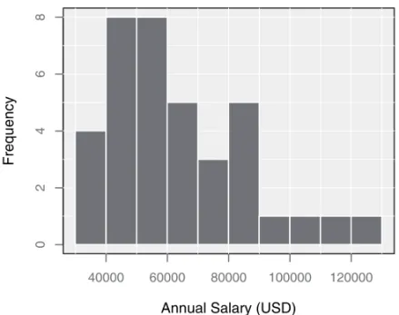
The histogram appears inFigure 1.3(in gray scale whereas the usual default involves color). We observe that the Salaries of these 37 employees range from below $40,000 to above $120,000, but most of the salaries are concentrated in the lower range, particularly between $40,000 and $60,000.
Annual Salary (USD)
Fre
qu
ency
40000 60000 80000 100000 120000
0246
8
Figure 1.3 The gray color themelessRhistogram for Salary from the Employee data set.
The Histogram function also generates text output shown in Listing 1.4. The summary summary statistics, Section 5.3.1, p. 105 statistics appear first: the total sample size, number of missing values, and the sample statistics of the mean, standard deviation, minimum, median and maximum. Also provided is a list of any outlier,
Section 5.3.1, p. 106 outliers and a frequency table based on all of the bins, along with the proportions, cumulative frequencies and cumulative proportions. Further discussion of this and other features of the Histogramfunction are deferred untilChapter 5.
Salary, Annual Salary (USD)
---n miss mean sd min mdn max
37 0 63795.557 21799.533 36124.970 59547.600 124419.230
Listing 1.4 Summary statistics of Salary.
Our goal has been accomplished, our first R/lessR data analysis. As shown in the next chapter, to do data analysis of data stored in your own data file use Read to locate and then read a data file that you store on your computer system. The version of Read for this task is simpler in this more common situation, with only an empty set of parentheses. The empty parentheses inform R to allow you to browse, that is, navigate, your computer file system to
locate the folder that contains your data file. libraryfunction, Section 1.3.1, p. 6 From the start of the Rsession to obtaining a histogram in color with various text output
requires two or three statements, depending on whether the library(lessR)statement had
previously been placed in the.Rprofilefile. OneRstatement obtains the input needed for the .Rpofile, p. 6 analysis, which is to read the data into theRdata tablemydata. Then enter just one statement
> library(lessR) > mydata <- Read() > Histogram(Salary)
Listing 1.5 R/lessRinstructions to generate a histogram of the variable Salary from a data file stored on the user’s computer system.
If no argument is passed to theHistogramfunction, then a histogram is generated foreach numerical variable in the data table, what Rcalls a data frame.
> Histogram()
The same result is obtained for both histograms and bar charts with the lessR function CountAll, again with no arguments.
CountAll function: Bar chart or histogram and summary statistics for all variables.
> CountAll()
Each histogram or bar chart is written to its ownpdf file and the corresponding statistical summaries are written to the R text window, the console. The lessR enhancements to R minimize the amount of work needed to accomplish data analysis and obtain meaningful, hopefully aesthetically pleasing results.
1.3.4 Quit
R
To end anRsession from the command line prompt, use the quit function, q. Quit function:
End anRsession.
R Input Quit R > q()
Or, when running within the Windows menu system, choose the menu sequence File ✄
Exit as with virtually any other Windows application. The same applies for the Macintosh sequenceR✄Quit R.
Unless the default settings have been changed, you are prompted after entering the quit command to save the working session, as shown inListing 1.6.
> q()
Save workspace image? [y/n/c]: n
Listing 1.6 The quitRdialog.
1.3.5
R
Functions
All work is done in R with functions. Call a function with some information that is then argumentsof a function: Information used by the function. processed by that function, such as data values for a function that processes data. The
information passed to a function, referenced in between the parentheses of the function call,
are the argumentsof the function. In our histogram example, the one argument passed to the default value: Assumed value for an argument of a function that can be explicitly changed. Histogramfunction is the variable name, Salary. Specifying the variable name as an argument
makes the data values for that variable accessible to the function.
Some arguments of a function havedefault values, which are assumed but can be overridden.
For example,lessRfunctions such as Histogramuse thedata argument to specify the name dataargument: The name of the data frame that contains the variables for analysis. of the data frame, R’s name for the data table that contains the variables of interest. The
default value for the input data frame is mydata, so the following two function calls are equivalent.
> Histogram(Salary) or > Histogram(Salary, data=mydata)
For ease of use rely upon the default. Usually only invoke thedataoption when the input data frame isnot mydata. If all the arguments in a function call are set to their default values, then no information needs to be passed to the function. The paired parentheses, however, are always part of the function call even if empty.
Functions may also have some arguments with no default value. These functions require the
values of these arguments to be explicitly specified. To see the full list of arguments and default ?function, the
standardRhelp
function, Section 1.3.2, p. 9 values for a function, along with other information, request the manual pages for the function.
To obtain these pages, enter the function name preceded by a question mark,?.
Types of Functions
There are at least three different types of functions within theRsystem.Utility functionsprovide
utilityfunction: Inform or set characteristics of the data processing environment. information or set characteristics of the overall environment to facilitate data processing. An
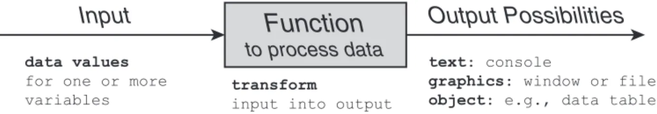
example of a utility function is theHelpfunction. Helpfunction, Section 1.3.2, p. 7 The two other types of functions process data as illustrated inFigure 1.4, such as thelessR
function Histogram. More specifically the type of data processing done by Histogramis data analysis. A data analysis function applies statistical methods to process the data to obtain the
data analysis function: Procedure to access and analyze data.
requested analysis, the output of the function. The Histogram function directs the resulting text output to the console and the graphics output to a graphics window.
Function
Input
Output Possibilities
transform
input into output
text: console
graphics: window or file object: e.g., data table data values
for one or more variables
to process data
Figure 1.4 General procedure for functions that process data, either data analysis or data modification.
As we discuss inChapters 2 and3, another way to process data is to create or modify the data in preparation for subsequent data analysis. One example of adata modification functionis
Read, which reads data from an external data file and then directs the output to anRdata table, usually named mydata as in the preceding example. Other examples of data modification are to sort the data, or to transform the data values of a variable such as by taking their logarithms. The modified data can then either be directed back to overwrite the original mydata, or to a new data table leaving the originalmydataunmodified.
The output from data analysis functions naturally involves numbers, which are displayed with a set level of decimal digits. By default lessRfunctions generally specify the number of digits.doption:
Explicitly set the number of decimal digits for the output.
displayed decimal digits as one more than the number of decimal digits for the input data values. Or two decimal digits are displayed if the input data values are all integers. If more or less decimal digits are desired, then specify with digits.d in the calls to the various lessR functions.
Suppress the text output to the console for the data modification functions and most other lessR functions with the quiet=TRUEoption included as part of the function call. With the quiet=TRUE
option: Suppress all text output to the console.
quietoption invoked these functions continue sending output to a special output object and/or a graphics window without sending any text to the console.
The primary purpose of some functions is to display text output to the console. Suppressing brief=TRUE
option: Reduce text output to the console.
their text output entirely is not meaningful. Instead the briefoption set to TRUEreduces the amount of output to just the minimum amount needed to convey the most basic results. Both thequietandbriefoptions can also be set system wide with the lessRfunction set. Then their values remain in effect for all subsequent analyses unless explicitly changed.
setfunction,
Section 1.4.1, p. 16
Standard
R
Functions
StandardRfunctions tend to be very specific in terms of their output. Many of these functions do not provide any output to the console but instead send a returned object back into the R environment as the primary output. After running the function, access the output objects to extract the needed information.
R functions do not have a default data source, so the data table must always be explicitly referenced. For example, the standard R function to obtain a histogram is hist. To use the function the data frame that contains the variables of interest must first be identified. Unfortunately, there is no consistent method to identify this information. AlllessRfunctions $ notation: One
application is to identify the relevant data frame.
use the data option to identify the relevant data table. Some standard R functions use this option, but most do not. One way to indicate the input data table for functions that do not use thedataoption is to use the$ notation to prefix the name of the data table to the variable name.
> hist(mydata$Salary)
withfunction:
Identify the relevant data frame.
Or, use theR withfunction to wrap around the function call.
> with(mydata, hist(Salary))
The resulting histogram has no default colors, no grid lines, and no text output. To obtain numerical output, assign the output of the function to an object, such ash.
Analysis of the h object provides information such as the counts for each bin. The information can be displayed at the console by entering h at the command prompt, but this information is more intended as input for additional programming than it is for consumption as finished output. Then useR statements to extract and then apply the additional programming such as to arrange the numerical output for display at the console. ManylessRfunctions also return the same object as the corresponding R function that provides the computations, such as theHistogramfunction that can return the same object as hist.
The kind of programming that accesses this information is not covered in this book because thelessRfunctions do this work for you. EachlessRdata analysis function runs one or more standard R functions, usually multiple functions, extracts the relevant information from each and then arranges and displays text output at the console and, if relevant, sends graphics to a graphics window. The standardRfunctions become a kind of tool kit thatlessRfunctions rely upon to construct their output.
1.3.6 Lists of Values
When using statistical software such asRa frequent task is to specify a list of variables, or a list of constants of either numbers or character strings. For example, suppose you wish to have the histogram bars filled with two alternating colors, here two shades of gray, defined on a scale
where "gray0" is black and "gray100"is white. The col.fill option specifies the color of col.filloption, Table 1.1, p. 17 the histogram bars.
> Histogram(Salary, col.fill=c("gray40","gray70"))
cfunction:
Combine a list of values. InRa list of individual values separated by commas is always enclosed in parentheses with thecfunction, which delineates a list of values from the rest of the information that surrounds the list.
Another example is the list of the first eight integers specified with thec function.
> c(1,2,3,4,5,6,7,8)
:notation: Specify
a sequential set of integers. If the items in the list are sequential the:notation can be used instead.
> 1:8
Or, the types of expressions for a list can be combined.
> c(1:4,5,6,7:8)
Enter any of the three preceding expressions at the command prompt to obtain the following output.
[1] 1 2 3 4 5 6 7 8
The concept of a list applies not only to a list of numbers as illustrated here but also to lists list of variables,
Section 8.3, p. 195 of variables.
1.4
R
Graphs
1.4.1 Color Themes
Graphics fromlessRfunctions are based on color themes, each with a pre-defined color palette. The default color theme isblue, so by default all graphs include color. This book is printed in color theme: A
set of related colors
for graphic output. gray scale (to save you money), so graphics here are printed with the gray scale color theme. The
chosen gray color theme follows Hadley Wickham’s design choices in his innovative graphics package ggplot2(Wickham, 2009).
In addition to blue and gray, other available color themes include green, gold, rose, red, purple, dodgerblue, sienna, white, orange.black, and gray.black. Most themes have lighter backgrounds, though any setting can be customized. The orange.black and gray.blackthemes have a black background by default.
setfunction: Select
a system option such as color theme and related color choices.
Use thelessRutility functionsetto change the theme for all subsequent graphics. Enclose the name of the color theme in quotes.
lessR Input Set color theme for subsequent analyses such as gray scale > set(colors="gray")
If you prefer a specific theme over the default blue, add this set statement to your .Rprofilefile to automatically invoke the preferred theme each timeRis started.
.Rprofile, p. 6 trans.fill.bar, trans.fill.pt options:
Transparency levels for the color of an interior of a bar or point.
The function set can also set the transparency of bars or points in a graph with the trans.fill.bar and trans.fill.pt options. The lessR default setting for the interior of plotted points istrans.fill.pt=0.66, a partial transparency. To plot points with a completely filled color, oblique, set the value of trans.fill.pt to 0. A value of 1 means complete transparency.
The default setting for filled rectangular regions such as the bars of a histogram is trans.fill.bar=0. That is, the default bars such as for a histogram are fully oblique. Set col.bg, col.grid
options: Set background color, grid color.
the background color and grid line colors with col.bgandcol.grid, respectively.2
The ghostoption creates a black background, removes grid lines, and adds a transparency level to the bars, such as for a histogram. The following function call sets the color theme in subsequent graphs to dodgerblue, turns on the ghostoption, and turns off the transparency of plotted points.
ghostoption: Create a ghost effect for the
graphics. > set(colors="dodgerblue", ghost=TRUE, trans.fill.pt=0)
1.4.2 Individual Colors
bars of a histogram or the points of a scatter plot. To view the available options for any one R helpfunction, Section 1.3.2, p. 9 graphics procedure, access help for that function by entering the function’s name proceeded by
a question mark.
Table 1.1 lists the color options available for most lessR graphics functions. Most of the graphicslessRfunctions usecol.fillandcol.stroketo define the interior of the relevant plotted object and its outline, respectively. For the histogram, these options refer to the color of the bars and the corresponding borders. For the plotted points in a scatter plot these options refer to the interior color of the points and their border color. Use theset function to set any of these colors to"transparent"to remove the color.
Table 1.1 Available color choices forlessRgraphics functions such asHistogramandScatterPlot.
Option Meaning
col.fill Color of bars or plotted points. col.stroke Color of the border of the bars. col.bg Color of the plot background. col.grid Color of the grid lines.
col.axis Color of the font used to label the axis values. col.ticks Color of the ticks used to label the axis values.
One way to specify an individual color is to specify one of the 657 color names inR(though some names are just different spellings for the same color). To view the colors invoke thelessR functionshowColors.
lessR Input Display a sample of each R named color > showColors()
showColors function: Create an illustrated listing of
all namedRcolors.
This function call generates apdf file that contains all the color names and also a sample of each color and its corresponding rgbcomposition, that is, its defining red, green, and blue component.
For example, there is a color named"aquamarine3", and a very pale color named"snow". The following produces a histogram of Salary with the current color theme but modified colors for the histogram bars and background of the graph.
> Histogram(Salary, col.fill="aquamarine3", col.bg="snow")
In addition to all of the named colors, a color can also be customized in terms of its location within a color space. For example the rgb function specifies a color precisely according to its red, green, and blue component.
ThemaxColorValue=255option indicates to scale the colors from 0 to 255, the same scale used by Adobe Photoshop and alsohtml, which forms the basis for web pages.
1.4.3 Axes Labels
If the data frame that contains the data for analysis contains thelessRfeature of variable labels, variable labels,
Section 2.4.1, p. 46
then these labels automatically become the corresponding axes labels on the resulting graph. Otherwise the default labels are the variable names. Custom labels for the horizontal or x-axis, xlab, ylab
options: Custom axis labels.
and the vertical or y-axis, are provided by thexlab andylaboptions, respectively. The graph title is set withmain.
mainoption:
Optional graph title.
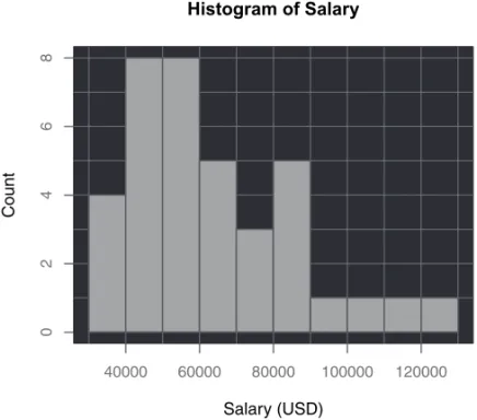
To illustrate, re-do the histogram from Figure 1.3 with customized labels and also with a different color theme. One possibility is to choose a color theme that provides a black color themes,
Section 1.4.1,
p. 16 background by default, optimized for viewing when projected on a large screen.
lessR Input
> set(colors="gray.black")
> Histogram(Salary, xlab="Salary (USD)", ylab="Count", main="Histogram of Salary")
The histogram displayed with this alternate color theme is in Figure 1.5. This color theme applies to all subsequent graphic output until explicitly changed, or until R is quit and then restarted.
Histogram of Salary
Salary (USD)
Co
u
nt
40000 60000 80000 100000 120000
0246
8
1.4.4 Save Graphs as
Files
After creating a graph such as a histogram, the graph can be saved to a file on your computer system. One option for Windows and Macintosh users is to right-click on the window that contains the graph, copy it and then paste it into the word processor that contains the report
of the analysis. Another option is to write the graph directly to a pdffile as it is generated. lessR Helpfunction, Section 1.3.2, p. 7 The lessR graphics functions provide a means to save the graph directly to a pdf file,
without interfering with any displayed help window from the lessR help system. Those pdf.fileoption:
pdffile for which
to direct alessR
function graphics output. routines such as theHistogramfunction that generate a single graph have an optionpdf.file that provide for the name of the resulting file. Accompanying options are pdf.width and pdf.heightto change the size of the graph from the default values of 5 inches by 5 inches.
lessR Input Generate and save the histogram directly to a pdf file
> Histogram(Salary, pdf.file="myHistogram.pdf", pdf.width=6)
pdfoption: Set to
TRUEto savepdf
files forlessR
functions that generate multiple graphics. Functions that generate multiple graphics, such as the Regression function, have a pdf
option that is set toTRUE to generate the graphics. In this situation each of the file names is automatically provided.
1.5
Reproducible Code
An analysis should be repeatable at some future time. To reproduce an analysis the code to
reproducible code: The instructions to generate an analysis can be repeated at some future time. generate the analysis must be able to be re-run, what is calledreproducible code. TheRstatements
to accomplish a specific analysis, such as inListing 1.5, should generally be saved in a standard text file so that these instructions are reproducible. Atext fileconsists of only standard characters, which consist of the upper and lowercase letters of the alphabet, digits, punctuation marks, and a few control codes. Text files are generally created with atext editor, a kind of simplified word
text file: A file that consists of only standard characters. processor that only works with the standard text characters.3
text editor: An editor for editing a text file. Several text editors integrate with theRenvironment so well that they become an extension
of R itself. Your author exclusively uses a non-traditional, free text editor vim, which runs on
Windows, Macintosh, Linux/Unix, iOS for the iPad and iPhone, and Android. An advantage of vim: General purpose text editor
with excellentR
compatibility. vimas a general text editor is that once having learned its insert and normal modes, and various
keystroke combinations for navigating and editing text, writing and editing text is considerably faster than with a traditional word processor.vimalso integrates with other environments. For example, this book was written withvimin conjunction with a powerful, cross-platform, open source and free typesetting systemLaTeX.
code integration: Transfer code entered into an editor to an environment for executing the
code, such asR.
Code integration, which transfers instructions fromvimdirectly toR, is one means by which vimintegrates withR. From withinvimone keystroke combination starts anRsession, or submits a single line, selected range of lines, or an entire file of Rinstructions directly into the running R session. All entering and editing of code takes place within a vim window, and all output flows into an adjacentR window.
Another form of integration of a text editor withRissyntax highlighting. Within the editor, Rkeywords are highlighted, as are numerical constants, quoted strings, and so forth, all usually in different colors. This highlighting makes the on-screen text considerably more readable and
1 library(lessR)
2 set(colors=“dodgerblue”, ghost=TRUE, trans.fill.pt=0) 3
4 Read() 5
6 Histogram(Salary, xlab=“Salary (USD)”, ylab=“Count”)
Figure 1.6 Excerpt ofRinstructions in thevimeditor with gray scale syntax highlighting.
Alternatives also exist for a more traditional editing experience than vim yet that still provide a free editing product with code integration and syntax highlighting. The recommended traditional style text editor for Macintoshs isTextWrangler. Windows users have theTinn-R editor and R development system that integrates with the R system, or the general purpose text editor and Notepad replacementNotepad++, with theNpptoRplug-in. Linux gnome users, as well as Windows and Macintosh users, have gedit with the RGedit plug-in. Many other Rstudio,
rstudio.com possibilities exist as well, including the full editing and development environment provided by
RStudio.
At a minimum, use a simple, basic text editor to develop and store your R programs. An editor that links directly to R is the most elegant solution, but even without linking to R directly you can manually copy and paste yourRinstructions from an editor intoR. Save yourR instructions gradually so as to build a library of instructions to accomplish a variety of analyses. With this strategy you can reproduce the output of any one analysis when desired, or do a simple modification to obtain a related analysis.
1.6
Data
Data analysis begins, naturally enough, with data. This section presents two sets of data analyzed throughout this book, and a discussion of the different types of variables typically encountered in data sets. The rest of this book shows how to read a data set into R for analysis and then conduct a variety of analyses.
1.6.1 Data Example I: Employee Data
The human resources department of a company recorded the following information for each employee: Name, Years of employment, Gender, Department employed, annual Salary, Satisfaction with work environment, and Health Plan. Data such as these are naturally organized data file: A file on
a computer system that contains data, usually organized into a table of rows and columns.
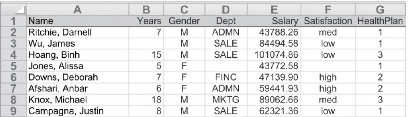
into a rectangular table for subsequent analysis. Consider a data file with measurements organized into a table for 37 employees, available on the web as an Excel worksheet.
http://lessRstats.com/data/employee.xlsx
Figure 1.7displays the first nine lines of the Excel version of this data file. unit of analysis:
The class of people, organizations, things or places from which measurements are obtained.
A basic characteristic of a data table is the unit of the analysis, the object of study. In this example the unit of analysis is a person, an employee at a specific company. Other potential units of analysis include organizations, places, events, or things in general.
Each cell of this table represents a single data value, the value of a variable for a specific instance of the unit of the analysis, here a specific person. For example, the person listed in the data value: The
value of a single measurement or