123
LNBIP 324
7th European Summer School, eBISS 2017
Bruxelles, Belgium, July 2–7, 2017
Tutorial Lectures
Business Intelligence
and Big Data
T
ut
in Business Information Processing
324
Series Editors
Wil van der AalstRWTH Aachen University, Aachen, Germany John Mylopoulos
University of Trento, Trento, Italy Michael Rosemann
Queensland University of Technology, Brisbane, QLD, Australia Michael J. Shaw
University of Illinois, Urbana-Champaign, IL, USA Clemens Szyperski
Business Intelligence
and Big Data
7th European Summer School, eBISS 2017
Bruxelles, Belgium, July 2
–
7, 2017
Tutorial Lectures
UniversitéLibre de Bruxelles Brussels
Belgium
ISSN 1865-1348 ISSN 1865-1356 (electronic) Lecture Notes in Business Information Processing
ISBN 978-3-319-96654-0 ISBN 978-3-319-96655-7 (eBook) https://doi.org/10.1007/978-3-319-96655-7
Library of Congress Control Number: 2018948636
©Springer International Publishing AG, part of Springer Nature 2018
This work is subject to copyright. All rights are reserved by the Publisher, whether the whole or part of the material is concerned, specifically the rights of translation, reprinting, reuse of illustrations, recitation, broadcasting, reproduction on microfilms or in any other physical way, and transmission or information storage and retrieval, electronic adaptation, computer software, or by similar or dissimilar methodology now known or hereafter developed.
The use of general descriptive names, registered names, trademarks, service marks, etc. in this publication does not imply, even in the absence of a specific statement, that such names are exempt from the relevant protective laws and regulations and therefore free for general use.
The publisher, the authors and the editors are safe to assume that the advice and information in this book are believed to be true and accurate at the date of publication. Neither the publisher nor the authors or the editors give a warranty, express or implied, with respect to the material contained herein or for any errors or omissions that may have been made. The publisher remains neutral with regard to jurisdictional claims in published maps and institutional affiliations.
The 7th European Business Intelligence and Big Data Summer School (eBISS 20171) took place in Brussels, Belgium, in July 2017. Tutorials were given by renowned experts and covered advanced aspects of business intelligence and big data. This volume contains the lecture notes of the summer school.
Thefirst chapter covers data profiling, which is the process of metadata discovery. This process involves activities that range from ad hoc approaches, such as eye-balling random subsets of the data or formulating aggregation queries, to systematic inference of metadata via profiling algorithms. The chapter emphasizes the importance of data profiling as part of any data-related use-case, classifying data profiling tasks, and reviews data profiling systems and techniques. The chapter also discusses hard prob-lems in data profiling, such as algorithms for dependency discovery and their appli-cation in data management and data analytics. It concludes with directions for future research in the area of data profiling.
The second chapter targets extract–transform–load (ETL) processes, which are used for extracting data, transforming them, and loading them into data warehouses. Most ETL tools use graphical user interfaces (GUIs), where the developer“draws”the ETLflow by connecting steps/transformations with lines. Although this gives an easy overview, it can be rather tedious and requires a lot of trivial work for simple things. This chapter proposes an alternative approach to ETL programming by writing code. It presents the Python-based framework pygrametl, which offers commonly used func-tionality for ETL development. By using the framework, the developer can efficiently create effective ETL solutions from which the full power of programming can be exploited. The chapter also discusses some of the lessons learned during the devel-opment of pygrametl as an open source framework.
The third chapter presents an overview of temporal data management. Despite the ubiquity of temporal data and considerable research on the processing of such data, database systems largely remain designed for processing the current state of some modeled reality. More recently, we have seen an increasing interest in the processing of temporal data. The SQL:2011 standard incorporates some temporal support, and commercial DBMSs have started to offer temporal functionality in a step-by-step manner. This chapter reviews state-of-the-art research results and technologies for storing, managing, and processing temporal data in relational database management systems. It starts by offering a historical perspective, after which it provides an over-view of basic temporal database concepts. Then the chapter surveys the state of the art in temporal database research, followed by a coverage of the support for temporal data in the current SQL standard and the extent to which the temporal aspects of the standard are supported by existing systems. The chapter ends by covering a recently
proposed framework that provides comprehensive support for processing temporal data and that has been implemented in PostgreSQL.
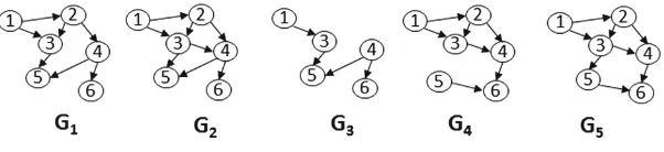
The fourth chapter discusses historical graphs, which capture the evolution of graphs through time. A historical graph can be modeled as a sequence of graph snapshots, where each snapshot corresponds to the state of the graph at the corresponding time instant. There is rich information in the history of the graph not present in only the current snapshot of the graph. The chapter presents logical and physical models, query types, systems, and algorithms for managing historical graphs.
Thefifth chapter introduces the challenges around data streams, which refer to data that are generated at such a fast pace that it is not possible to store the complete data in a database. Processing such streams of data is very challenging. Even problems that are highly trivial in an off-line context, such as:“How many different items are there in my database?”become very hard in a streaming context. Nevertheless, in the past decades several clever algorithms were developed to deal with streaming data. This chapter covers several of these indispensable tools that should be present in every big data scientist’s toolbox, including approximate frequency counting of frequent items, car-dinality estimation of very large sets, and fast nearest neighbor search in huge data collections.
Finally, the sixth chapter is devoted to deep learning, one of the fastest growing areas of machine learning and a hot topic in both academia and industry. Deep learning constitutes a novel methodology to train very large neural networks (in terms of number of parameters), composed of a large number of specialized layers that are able to represent data in an optimal way to perform regression or classification tasks. The chapter reviews what is a neural network, describes how we can learn its parameters by using observational data, and explains some of the most common architectures and optimizations that have been developed during the past few years.
In addition to the lectures corresponding to the chapters described here, eBISS 2017 had an additional lecture:
– Christoph Quix from Fraunhofer Institute for Applied Information Technology, Germany:“Data Quality for Big Data Applications”
This lecture has no associated chapter in this volume.
As with the previous editions, eBISS joined forces with the Erasmus Mundus IT4BI-DC consortium and hosted its doctoral colloquium aiming at community building and promoting a corporate spirit among PhD candidates, advisors, and researchers of different organizations. The corresponding two sessions, each organized in two parallel tracks, included the following presentations:
– Isam Mashhour Aljawarneh,“QoS-Aware Big Geospatial Data Processing” – Ayman Al-Serafi,“The Information Profiling Approach for Data Lakes”
– Katerina Cernjeka,“Data Vault-Based System Catalog for NoSQL Store Integration in the Enterprise Data Warehouse”
– Daria Glushkova,“MapReduce Performance Models for Hadoop 2.x”
– Muhammad Idris, “Active Business Intelligence Through Compact and Efficient Query Processing Under Updates”
– Hiba Khalid,“Meta-X: Discovering Metadata Using Deep Learning” – Elvis Koci,“From Partially Structured Documents to Relations” – Rohit Kumar,“Mining Simple Cycles in Temporal Network”
– Jose Miguel Mota Macias,“VEDILS: A Toolkit for Developing Android Mobile Apps Supporting Mobile Analytics”
– Rana Faisal Munir,“A Cost-Based Format Selector for Intermediate Results” – Sergi Nadal,“An Integration-Oriented Ontology to Govern Evolution in Big Data
Ecosystems”
– Dmitriy Pochitaev, “Partial Data Materialization Techniques for Virtual Data Integration”
– Ivan Ruiz-Rube,“A BI Platform for Analyzing Mobile App Development Process Based on Visual Languages”
We would like to thank the attendees of the summer school for their active par-ticipation, as well as the speakers and their co-authors for the high quality of their contribution in a constantly evolving and highly competitive domain. Finally, we would like to thank the external reviewers for their careful evaluation of the chapters.
The 7th European Business Intelligence and Big Data Summer School (eBISS 2017) was organized by the Department of Computer and Decision Engineering (CoDE) of the UniversitéLibre de Bruxelles, Belgium.
Program Committee
Alberto Abelló Universitat Politècnica de Catalunya, BarcelonaTech, Spain
Nacéra Bennacer Centrale-Supélec, France
Ralf-Detlef Kutsche Technische Universität Berlin, Germany Patrick Marcel UniversitéFrançois Rabelais de Tours, France Esteban Zimányi UniversitéLibre de Bruxelles, Belgium
Additional Reviewers
Christoph Quix Fraunhofer Institute for Applied Information Technology, Germany
Oscar Romero Universitat Politècnica de Catalunya, BarcelonaTech, Spain
Alejandro Vaisman Instituto Tecnológica de Buenos Aires, Argentina Stijn Vansummeren Universitélibre de Bruxelles, Belgium
Panos Vassiliadis University of Ioannina, Greece
Hannes Vogt Technische Universität Dresden, Germany Robert Wrembel Poznan University of Technology, Poland
Sponsorship and Support
An Introduction to Data Profiling . . . 1 Ziawasch Abedjan
Programmatic ETL . . . 21 Christian Thomsen, Ove Andersen, Søren Kejser Jensen,
and Torben Bach Pedersen
Temporal Data Management–An Overview . . . 51 Michael H. Böhlen, Anton Dignös, Johann Gamper,
and Christian S. Jensen
Historical Graphs: Models, Storage, Processing. . . 84 Evaggelia Pitoura
Three Big Data Tools for a Data Scientist’s Toolbox . . . 112 Toon Calders
Let’s Open the Black Box of Deep Learning! . . . 134 Jordi Vitrià
Ziawasch Abedjan(B)
TU Berlin, Berlin, Germany [email protected]
Abstract. One of the crucial requirements before consuming datasets for any application is to understand the dataset at hand and its meta-data. The process of metadata discovery is known as data profiling. Profiling activities range from ad-hoc approaches, such as eye-balling random subsets of the data or formulating aggregation queries, to sys-tematic inference of metadata via profiling algorithms. In this course, we will discuss the importance of data profiling as part of any data-related use-case, and shed light on the area of data profiling by classifying data profiling tasks and reviewing the state-of-the-art data profiling systems and techniques. In particular, we discuss hard problems in data profil-ing, such as algorithms for dependency discovery and their application in data management and data analytics. We conclude with directions for future research in the area of data profiling.
1
Introduction
Recent studies show that data preparation is one of the most time-consuming tasks of researchers and data scientists1. A core task for preparing datasets is profiling a dataset. Data profiling is the set of activities and processes to determine the metadata about a given dataset [1]. Most readers probably have engaged in the activity of data profiling, at least by eye-balling spreadsheets, database tables, XML files, etc. Possibly more advanced techniques were used, such as keyword-searching in datasets, writing structured queries, or even using dedicated analytics tools.
According to Naumann [46], data profiling encompasses a vast array of meth-ods to examine datasets and produce metadata. Among the simpler results are statistics, such as the number of null values and distinct values in a column, its data type, or the most frequent patterns of its data values. Metadata that are more difficult to compute involve multiple columns, such as inclusion depen-dencies or functional dependepen-dencies. Also of practical interest are approximate versions of these dependencies, in particular because they are typically more efficient to compute. This chapter will strongly align with the survey published in 2015 on profiling relational data [1] and will focus mainly on exact methods. Note that all discussed examples are also taken from this survey.
1 https://www.forbes.com/sites/gilpress/2016/03/23/data-preparation-most-time-consuming-least-enjoyable-data-science-task-survey-says/#2c61c6c56f63. c
Springer International Publishing AG, part of Springer Nature 2018 E. Zim´anyi (Ed.): eBISS 2017, LNBIP 324, pp. 1–20, 2018.
Apart from managing the input data, data profiling faces two significant challenges:(i) performing the computation, and(ii) managing the output. The first challenge is the main focus of this chapter and that of most research in the area of data profiling: The computational complexity of data profiling algorithms depends on the number or rows and on the number of columns. Often, there is an exponential complexity in the number of columns and subquadratic complexity in the number of rows. The second challenge, namely meaningfully interpreting the data profiling has yet to be addressed. Profiling algorithms generate data and often the amount of data itself is impractical requiring a meta-profiling step, i.e., interpretation, which is usually performed by database and domain experts.
1.1 Use Cases for Data Profiling
Statistics about data and dependencies are have always been useful in query optimization [34,41,52]. Furthermore, data profiling plays an important role in use cases, such as data exploration, data integration, and data analytics.
Data Exploration. Users are often confronted with new datasets, about which they know nothing. Examples include data files downloaded from the Web, old database dumps, or newly gained access to some DBMS. In many cases, such data have no known schema, no or old documentation, etc. Even if a formal schema is specified, it might be incomplete, for instance specifying only the primary keys but no foreign keys. A natural first step is to identify the basic structure and high-level content of a dataset. Thus, automated data profiling is needed to provide a basis for further analysis. Morton et al. recognize that a key challenge is overcoming the current assumption of data exploration tools that data is “clean and in a well-structured relational format” [45].
Data Integration and Data Cleaning. There are crucial questions to be answered before different data sources can be integrated: In particular, the dimensions of a dataset, its data types and formats are important to recognize before auto-mated integration routines can be applied. Similarly, profiling can help to detect data quality problems, such as inconsistent formatting within a column, missing values, or outliers. Profiling results can also be used to measure and monitor the general quality of a dataset, for instance by determining the number of records that do not conform to previously established constraints [35]. Generated con-straints and dependencies also allow for rule-based data imputation.
1.2 Chapter Overview
The goal of this chapter is to provide an overview on existing algorithms and open challenges in data profiling. The remainder of this chapter is organized as follows. In Sect.2, we outline and define data profiling based on a new taxonomy of profiling tasks and briefly survey the state of the art of the two main research areas in data profiling: analysis of single and multiple columns. We dedicate Sect.3 on the detection of dependencies between columns. In Sect.4 we shed some light on data profiling tools from research and industry and we conclude this chapter in Sect.5.
2
Classification of Profiling Tasks
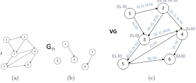
This section presents a classification of data profiling tasks according to the aforementioned survey [1]. Figure1shows the classification, which distinguishes single-column tasks, multi-column tasks, and dependency detection. While dependency detection falls under multi-column profiling, we chose to assign a separate profiling class to this large, complex, and important set of tasks.
2.1 Single Column Profiling
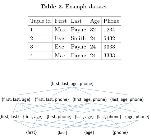
Typically, the generated metadata from single columns comprises various counts, such as the number of values, the number of unique values, and the number of non-null values. These metadata are often part of the basic statistics gathered by the DBMS. In addition, the maximum and minimum values are discovered and the data type is derived (usually restricted to string vs. numeric vs. date). More advanced techniques create histograms of value distributions and identify typical patterns in the data values in the form of regular expressions [54]. Table1 lists the possible and typical metadata as a result of single-column data profiling. In the following, we point out some of the interesting tasks.
From the number of distinct values theuniquenesscan be calculated, which is typically defined as the number of unique values divided by the number of rows. Apart from determining the exact number of distinct values, query optimization is a strong incentive to estimate those counts in order to predict query execu-tion plan costs without actually reading the entire data. Because approximate profiling is not the focus of this survey, we give only two exemplary pointers. Haas et al. base their estimation on data samples. They describe and empirically compare various estimators from the literature [27]. Another approach is to scan the entire data but use only a small amount of memory to hash the values and estimate the number of distinct values [6].
Theconstancy of a column is defined as the ratio of the frequency of the most frequent value (possibly a pre-defined default value) and the overall number of values. It thus represents the proportion of some constant value compared to the entire column.
Da
Fig. 1.A classification of traditional data profiling tasks according to [1].
distribution of the first digit d of a number approximately follows P(d) = log10(1 +1d) [8]. Thus, the 1 is expected to be the most frequent leading digit,
followed by 2, etc. Benford’s law has been used to uncover accounting fraud and other fraudulently created numbers.
2.2 Multi-column Profiling
Table 1.Overview of selected single-column profiling tasks [1]
Category Task Description
Cardinalities num-rows Number of rows
value lengthMeasurements of value lengths (minimum, maximum, median, and average)
null values Number or percentage of null values
distinct Number of distinct values; sometimes called “cardinality”
uniqueness Number of distinct values divided by the number of rows
Value distributions
histogram Frequency histograms (equi-width, equi-depth, etc.)
constancy Frequency of most frequent value divided by number of rows
quartiles Three points that divide the (numeric) values into four equal groups
first digit Distribution of first digit in numeric values; to check Benford’s law
Patterns basic type Generic data type, such as numeric, alphabetic, alphanumeric, date, time
data types data type Concrete DBMS-specific data type, such as varchar, timestamp, etc.
and domains size Maximum number of digits in numeric values
decimals Maximum number of decimals in numeric values
patterns Histogram of value patterns (Aa9. . . )
data class Semantic, generic data type, such as code, indicator, text, date/time, quantity, identifier
domain Classification of semantic domain, such as credit card, first name, city, phenotype
such as key or functional dependency discovery, also relates to multi-column profiling, we dedicate a separate section to dependency discovery as described in the next section.
Correlations and Association Rules. Correlation analysis reveals related numeric columns, e.g., in an Employees table,ageandsalarymay be correlated. A straightforward way to do this is to compute pairwise correlations among all pairs of columns. In addition to column-level correlations, value-levelassociations
may provide useful data profiling information.
association rule {bread} → {butter}, for example, states that if a transaction includes bread, it is also likely to include butter, i.e., customers who buy bread also buy butter. A set of items is referred to as anitemset, and an association rule specifies an itemset on the left-hand-side and another itemset on the right-hand-side.
Most algorithms for generating association rules from data decompose the problem into two steps [5]:
1. Discover all frequent itemsets, i.e., those whose frequencies in the dataset (i.e., theirsupport) exceed some threshold. For instance, the itemset{bread, butter}may appear in 800 out of a total of 50,000 transactions for a support of 1.6%.
2. For each frequent itemseta, generate association rules of the forml→a−l withl ⊂a, whose confidence exceeds some threshold. Confidence is defined as the frequency ofadivided by the frequency ofl, i.e., the conditional prob-ability ofl given a−l. For example, if the frequency of{bread, butter} is 800 and the frequency of {bread} alone is 1000 then the confidence of the association rule{bread} → {butter} is 0.8.
The first step is the bottleneck of association rule discovery due to the large number of possible frequent itemsets (or patterns of values) [31]. Popular algo-rithms for efficiently discovering frequent patterns include Apriori [5], Eclat [62], and FP-Growth [28]. Negative correlation rules, i.e., those that identify attribute values that do not co-occur with other attribute values, may also be useful in data profiling to find anomalies and outliers [11]. However, discovering negative association rules is more difficult, becauseinfrequent itemsets cannot be pruned the same way as frequent itemsets.
Clustering and Outlier Detection. Another useful profiling task is to iden-tify homogeneous groups of records as clusters or to ideniden-tify outlying records that do not fit into any cluster. For example, Dasu et al. cluster numeric columns and identify outliers in the data [17]. Furthermore, based on the assumption that data glitches occur across attributes and not in isolation [9], statistical inference has been applied to measure glitch recovery in [20].
Summaries and Sketches. Besides clustering, another way to describe data is to create summaries or sketches [13]. This can be done by sampling or hashing data values to a smaller domain. Sketches have been widely applied to answering approximate queries, data stream processing and estimating join sizes [18,23]. Cormode et al. give an overview of sketching and sampling for approximate query processing [15].
distinct value sets of columns A and B are not available, we can estimate the Jaccard similarity using theirMinHash signatures [19].
2.3 Dependencies
Dependencies are metadata that describe relationships among columns. In con-trast to multi-column profiling, the goal is to identify meta-data that describe relationships among column combinations and not the value combinations within the columns.
One of the common goals of data profiling is to identify suitable keys for a given table. Thus, the discovery of unique column combinations, i.e., sets of columns whose values uniquely identify rows, is an important data profiling task [29]. A unique that was explicitly chosen to be the unique record identifier while designing the table schema is called primary key. Since the discovered uniqueness constraints are only valid for a relational instance at a specific point of time, we refer to uniques and non-uniques instead of keys and non-keys. A further distinction can be made in terms of possible keys and certain keys when dealing with uncertain data and NULL values [37].
Another frequent real-world use-case of dependency discovery is the discov-ery of foreign keys [40] with the help of inclusion dependencies [7,42]. An inclu-sion dependency states that all values or value combinations from one set of columns also appear in the other set of columns – a prerequisite for a foreign key. Finally, functional dependencies (Fds) are relevant for many data quality
applications. A functional dependency states that values in one set of columns functionally determine the value of another column. Again, much research has been performed to automatically detectFds [32]. Section3 surveys dependency
discovery algorithms in detail.
2.4 Conditional, Partial, and Approximate Solutions
Real datasets usually contain exceptions to rules. To account for this, dependen-cies and other constraints detected by data profiling can be be relaxed. Typi-cally, relaxations in terms of partial and conditional dependencies have been the focus of research [12]. Within the scope of this chapter, we will only discuss the approaches for discovering the exact set of dependencies.
Partial dependencies are dependencies that hold for only a subset of the records, for instance, for 95% of the records or for all but 5 records. Such depen-dencies are especially valuable in cleaning dirty datasets where some records might be broken and impede the detection of a dependency. Violating records can be extracted and cleansed [57].
Conditional dependenciescan specify condition for partial dependencies. For instance, a conditional unique column combination might state that the col-umn city is unique for all records withCountry =‘USA’. Conditional inclusion dependencies (Cinds) were proposed by Bravo et al. for data cleaning and
con-textual schema matching [10]. Conditional functional dependencies (Cfds) were
Approximate dependenciesare not guaranteed to hold for the entire relation. Such dependencies are discovered using approximate solutions, such as sam-pling [33] or other summarization techniques [15]. Approximate dependencies can be used as input to the more rigorous task of detecting true dependencies. This survey does not discuss such approximation techniques.
2.5 Data Profiling vs. Data Mining
Generally, it is apparent that some data mining techniques can be used for data profiling. Rahm and Do distinguish data profiling from data mining by the num-ber of columns that are examined: “Data profiling focusses on the instance analy-sis of individual attributes. [. . . ] Data mining helps discover specific data patterns in large datasets, e.g., relationships holding between several attributes” [53]. While this distinction is well-defined, we believe several tasks, such as Ind or Fddetection, belong to data profiling, even if they discover relationships between
multiple columns.
The profiling survey [1] rather adheres to the following way of differentiation: Data profiling gathers technical metadata (information about columns) to sup-port data management; data mining and data analytics discovers non-obvious results (information about the content) to support business management with new insights. With this distinction, we concentrate on data profiling and put aside the broad area of data mining, which has already received unifying treat-ment in numerous textbooks and surveys [58].
3
Dependency Detection
Before discussing actual algorithms for dependency discovery, we will present a set of formalism that are used in the following. Then, we will present algo-rithms for the discovery of the prominent dependencies unique column combina-tions (Sect.3.1), functional dependencies (Sect.3.2), and inclusion dependencies (Sect.3.3). Apart from algorithms for these traditional dependencies, newer types of dependencies have also been the focus of research. We refer the reader to the survey on relaxed dependencies for further reading [12].
Notation. R and S denote relational schemata, with r and s denoting the instances of R and S, respectively. We refer to tuples of r and s as ri and
sj, respectively. Subsets of columns are denoted by upper-caseX, Y, Z(with|X|
denoting the number of columns in X) and individual columns by upper-case A, B, C. Furthermore, we define πX(r) andπA(r) as the projection ofr on the
attribute setX or attributeA, respectively; thus,|πX(r)| denotes the count of
distinct combinations of the values ofX appearing inr. Accordingly,ri[A]
indi-cates the value of the attributeAof tupleri andri[X] =πX(ri). We refer to an
3.1 Unique Column Combinations and Keys
Given a relation Rwith instancer, a unique column combination (a “unique”) is a set of columns X ⊆ R whose projection on r contains only unique value combinations.
Definition 1 (Unique/Non-Unique). A column combination X ⊆ R is a
unique, iff ∀ri, rj ∈ r, i = j : ri[X] = rj[X]. Analogously, a set of columns
X ⊆Ris a non-unique column combination(a “non-unique”), iff its projection on rcontains at least one duplicate value combination.
Each superset of a unique is also unique while each subset of a non-unique is also a non-unique. Therefore, discovering all uniques and non-uniques can be reduced to the discovery of minimal uniques and maximal non-uniques:
Definition 2 (Minimal Unique/Maximal Non-Unique). A column com-binationX ⊆Ris a minimal unique, iff∀X′⊂X :X′ is a non-unique.
Accord-ingly, a column combination X⊆R is a maximal non-unique, iff∀X′ ⊃X :X′
is a unique.
To discover all minimal uniques and maximal non-uniques of a relational instance, in the worst case, one has to visit all subsets of the given relation. Thus, the discovery of all minimal uniques and maximal non-uniques of a relational instance is an NP-hard problem and even the solution set can be exponential [26]. Given|R|, there can be||RR||
2
≥2|R2| minimal uniques in the worst case, i.e.,
as all combinations of size |R2|.
Gordian – Row-Based Discovery. Row-based algorithms require multiple runs over all column combinations as more and more rows are considered. They benefit from the intuition that non-uniques can be detected without verifying every row in the dataset.Gordian[56] is an algorithm that works this way in a
recursive manner. The algorithm consists of three stages: (i)Organize the data in form of a prefix tree, (ii) Discover maximal non-uniques by traversing the prefix tree,(iii) Generate minimal uniques from maximal non-uniques.
Each level of the prefix tree represents one column of the table whereas each branch stands for one distinct tuple. Tuples that have the same values in their prefix share the corresponding branches. E.g., all tuples that have the same value in the first column share the same node cells. The time to create the prefix tree depends on the number of rows, therefore this can be a bottleneck for very large datasets. However because of the tree structure, the memory footprint will be smaller than the original dataset. By a depth-first traversal of the tree for discovering maximum repeated branches, which constitute maximal non-uniques, maximal non-uniques will be discovered.
After discovering all maximal non-uniques,Gordiancomputes all minimal
The generation of minimal uniques from maximal non-uniques can be a bot-tleneck if there are many maximal non-uniques. Experiments showed that in most cases the unique generation dominates the runtime [2].
Column-Based Traversal of the Column Lattice. In the spirit of the well-known Apriori approach, minimal unique discovery working bottom-up as well as top-down can follow the same approach as for frequent itemset mining [5]. With regard to the powerset lattice of a relational schema, the Apriori algorithms generate all relevant column combinations of a certain size and verify those at once. Figure2illustrates the powerset lattice for the running example in Table2. The effectiveness and theoretical background of those algorithms is discussed by Giannela and Wyss [24]. They presented three breadth-first traversal strategies: a bottom-up, a top-down, and a hybrid traversal strategy.
Table 2.Example dataset.
Tuple id First Last Age Phone 1 Max Payne 32 1234 2 Eve Smith 24 5432 3 Eve Payne 24 3333 4 Max Payne 24 3333
Fig. 2.Powerset lattice for the example Table2[1].
Bottom-up unique discovery traverses the powerset lattice of the schema R from the bottom, beginning with all 1-combinations toward the top of the lattice, which is the |R|-combination. The prefixed numberk of k-combination
indicates the size of the combination. The same notation applies fork-candidates,
If the candidate is verified as unique, its minimality has to be checked. The algorithm terminates when k =|1-non-uniques|. A disadvantage of this candi-date generation technique is that redundant uniques and duplicate candicandi-dates are generated and tested.
The Apriori idea can also be applied to the top-down approach. Having the set of identified k-uniques, one has to verify whether the uniques are minimal. Therefore, for eachk-unique, all possible (k−1)-subsets have to be generated and verified. Experiments have shown that in most datasets, uniques usually occur in the lower levels of the lattice, which favours bottom-up traversal [2]. Hcais
an improved version of the bottom-up Apriori technique [2], which optimizes the candidate generation step, applies statistical pruning, and considers functional dependencies that have been inferred on the fly.
DUCC – Traversing the Lattice via Random Walk. While the breadth-first approach for discovering minimal uniques gives the most pruning, a depth-first approach might work well if there are relatively few minimal uniques that are scattered on different levels of the powerset lattice. Depth-first detection of unique column combinations resembles the problem of identifying the most promising paths through the lattice to discover existing minimal uniques and avoid unnecessary uniqueness checks. Ducc is a depth-first approach that
tra-verses the lattice back and forth based on the uniqueness of combinations [29]. Following a random walk principle by randomly adding columns to non-uniques and removing columns from uniques,Ducctraverses the lattice in a manner that
resembles the border between uniques and non-uniques in the powerset lattice of the schema.
Ducc starts with a seed set of2-non-uniques and picks a seed at random.
Eachk-combination is checked using the superset/subset relations and pruned if any of them subsumes the current combination. If no previously identified com-bination subsumes the current comcom-binationDuccperforms uniqueness
verifica-tion. Depending on the verification, Duccproceeds with an unchecked (k−
1)-subset or (k−1)-superset of the currentk-combination. If no seeds are available, it checks whether the set of discovered minimal uniques and maximal non-uniques correctly complement each other. If so,Duccterminates; otherwise, a new seed
set is generated by complementation.
Duccalso optimizes the verification of minimal uniques by using a position
list index (PLI) representation of values of a column combination. In this index, each position list contains the tuple IDs that correspond to the same value combination. Position lists with only one tuple ID can be discarded, so that the position list index of a unique contains no position lists. To obtain the PLI of a column combination, the position lists in PLIs of all contained columns have to be cross-intersected. In fact,Duccintersects two PLIs similar to how a hash
join operator would join two relations. As a result of using PLIs,Ducccan also
apply row-based pruning, because the total number of positions decreases with the size of column combinations. SinceDucc combines row-based and
3.2 Functional Dependencies
A functional dependency (Fd) over R is an expression of the form X → A,
indicating that ∀ri, rj ∈r ifri[X] =rj[X] thenri[A] =rj[A]. That is, any two
tuples that agree onX must also agree on A. We refer toX as the left-hand-side (LHS) and A as the right-hand-side (RHS). Given r, we are interested in finding all nontrivial and minimalFdsX →Athat hold onr, with non-trivial
meaningA∩X=∅and minimal meaning that there must not be anyFdY →A
for any Y ⊂X. A naive solution to theFd discovery problem is to verify for
each possible RHS and LHS combination whether there exist two tuples that violate the Fd. This is prohibitively expensive: for each of the|R|possibilities
for the RHS, it tests 2(|R|−1)possibilities for the LHS, each time having to scan rmultiple times to compare all pairs of tuples. However, notice that forX →A to hold, the number of distinct values ofX must be the same as the number of distinct values ofXA– otherwise at least one combination of values ofX that is associated with more than one value ofA, thereby breaking theFd[32]. Thus,
if we pre-compute the number of distinct values of each combination of one or more columns, the algorithm simplifies to:
Recall Table2. We have |πphone(r)| = |πage,phone(r)| = |πlast,phone(r)|. Thus, phone → age and phone → last hold. Furthermore, |πlast,age(r)| =
|πlast,age,phone(r)|, implying{last,age} →phone.
This approach still requires to compute the distinct value counts for all pos-sible column combinations. Similar to unique discovery,Fddiscovery algorithms
employ row-based (bottom-up) and column-based (top-down) optimizations, as discussed below.
Column-Based Algorithms. As was the case with uniques, Apriori-like approaches can help prune the space of Fds that need to be examined, thereby
optimizing the first two lines of the above straightforward algorithms. TANE [32], FUN [47], and FD Mine [61] are three algorithms that follow this strategy, with FUN and FD Mine introducing additional pruning rules beyond TANE’s based on the properties of Fds. They start with sets of single columns in the LHS
and work their way up the powerset lattice in alevel-wise manner. Since only minimalFds need to be returned, it is not necessary to test possibleFds whose
LHS is a superset of an already-found Fd with the same RHS. For instance,
in Table2, once we find that phone → age holds, we do not need to consider
{first,phone} →age,{last,phone} →age, etc.
Additional pruning rules may be formulated from Armstrong’s axioms, i.e., we can prune from consideration those Fds that are logically implied by those
we have found so far. For instance, if we find that A → B and B → A, then we can prune all LHS column sets including B, because A and B are equiva-lent [61]. Another pruning strategy is to ignore columns sets that have the same number of distinct values as their subsets [47]. Returning to Table2, observe that phone→firstdoes not hold. Since |πphone(r)|=|πlast,phone(r)|=|πage,phone(r)|=
a validFdwithfirston the RHS. To determine these cardinalities the approaches
use the PLIs as discussed in Sect.3.1.
Row-Based Algorithms. Row-based algorithms examine pairs of tuples to determine LHS candidates. Dep-Miner [39] and FastFDs [59] are two examples; the FDEP algorithm [22] is also row-based, but the way it ultimately findsFds
that hold is different.
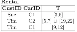
The idea behind row-based algorithms is to compute the so-called difference sets for each pair of tuples that are the columns on which the two tuples differ. Table3 enumerates the difference sets in the data from Table2. Next, we can find candidate LHS’s from the difference sets as follows. Pick a candidate RHS, say, phone. The difference sets that include phone, with phone removed, are:
{first,last,age},{first,age},{age},{last} and {first,last}. This means that there exist pairs of tuples with different values of phone and also with different val-ues of these five difference sets. Next, we find minimal subsets of columns that have a non-empty intersection with each of these difference sets. Such subsets are exactly the LHSs of minimal Fds with phone as the RHS: if two tuples
have different values of phone, they are guaranteed to have different values of the columns in the above minimal subsets, and therefore they do not cause
Fd violations. Here, there is only one such minimal subset, {last,age}, giving
{last,age} →phone. If we repeat this process for each possible RHS, and com-pute minimal subsets corresponding to the LHS’s, we obtain the set of minimal
Fds.
Table 3.Difference sets computed from Table2.[1]
Tuple ID pair Difference set
(1,2) first, last, age, phone
(1,3) first, age, phone
(1,4) age, phone
(2,3) last, phone
(2,4) first, last, phone
(3,4) first
Experiments confirm that row-based approaches work well on high-dimensional tables with a relatively small number of tuples, while column-based approaches perform better on low-dimensional tables with a large number of rows [49]. Recent approaches toFddiscovery are DFD [3] and HyFD [51]. DFD
decomposes the attribute lattice into|R|lattices, considering each attribute as a possible RHS of an Fd. On each lattice, DFD applies a random walk
app-roach by pruning supersets of Fd LHS’s and subsets of non-Fd LHS’s. HyFD
3.3 Inclusion Dependencies
An inclusion dependency (Ind) R.A ⊆S.B asserts that each value of column
A from relation R appears in column B from relation S; orA ⊆ B when the relations are clear from context. Similarly, for two sets of columns X and Y, we write R.X ⊆ S.Y, or X ⊆ Y, when each distinct value combination in X appears inY. We refer toR.AorR.X as the LHS andS.BorS.Y as the RHS.
Inds with a single-column LHS and RHS are referred to asunaryand those with
multiple columns in the LHS and RHS are calledn-ary. A naive solution toInd
discovery in relation instances rand sis to try to match each possible LHSX with each possible RHS Y. For any consideredX and Y, we can stop as soon as we find a value combination ofX that does not appear inY. This is not an efficient approach as it repeatedly scansrands when testing the possible LHS and RHS combinations.
Generating Unary Inclusion Dependencies. To discover unary Inds, a
common approach is to pre-process the data to speed up the subsequent Ind
discovery [7,43]. The SPIDER algorithm [7] pre-processes the data by sorting the values of each column and writing them to disk. Next, each sorted stream, corresponding to the values of one particular attribute, is consumed in parallel in a cursor-like manner, and anIndA⊆B can be discarded as soon as a value
in Ais read that is not present inB.
Generating n-ary Inclusion Dependencies. After discovering unaryInds,
a level-wise algorithm, similar to the TANE algorithm for Fd discovery can
be used to discover n-ary Inds. De Marchi et al. [43] propose an algorithm
that constructsInds withi columns from those withi−1 columns.
Addition-ally, hybrid algorithms have been proposed in [38,44] that combine bottom-up and top-down traversal for additional pruning. Recently, theBinderalgorithm,
which uses divide and conquer principles to handle larger datasets, has been introduced [50]. In the divide step, it splits the input dataset horizontally into partitions and vertically into buckets with the goal to fit each partition into main memory. In the conquer step, Binder then validates the set of all
pos-sible inclusion dependency candidates. Processing one partition after another, the validation constructs two indexes on each partition, a dense index and an inverted index, and uses them to efficiently prune invalid candidates from the result set.
Generating Foreign Keys. Ind discovery is the initial step for foreign key
detection: a foreign key must satisfy the corresponding inclusion dependency but not all Inds are foreign keys. For example, multiple tables may contain
auto-increment columns that serve as keys, and while inclusion dependencies among them may exist, they are not foreign keys. Once Inds have been discovered,
additional heuristics have been proposed, which essentially rank the discovered
Inds according to their likelihood of being foreign keys [40,55]. A very simple
4
Profiling Tools
To allow a more powerful and integrated approach to data profiling, software companies have developed data profiling techniques, mostly to profile data resid-ing in relational databases. Most profilresid-ing tools so far are part of a larger software suite, either for data integration or for data cleansing. We first give an overview of tools that were created in the context of a research project (see Table4 for a listing). Then we give a brief glimpse of the vast set of commercial tools with profiling capabilities.
Table 4.Research tools with data profiling capabilities [1].
Tool Main goal Profiling capabilities
Bellman [19] Data quality browser Column statistics, column similarity, candidate key discovery Potters Wheel [54] Data quality, ETL Column statistics (including value
patterns)
Data Auditor [25] Rule discovery CfdandCinddiscovery RuleMiner [14] Rule discovery Denial constraint discovery MADLib [30] Machine learning Simple column statistics
Research Prototypes. Data profiling tools are often embedded in data clean-ing systems. For example, the Bellman [19] data quality browser supports column analysis (counting the number of rows, distinct values, and NULL values, find-ing the most frequently occurrfind-ing values, etc.), and key detection (up to four columns). It also provides a column similarity functionality that finds columns whose value or n-gram distributions are similar; this is helpful for discovering potential foreign keys and join paths. Furthermore, it is possible to profile the evolution of a database using value distributions and correlations [18]: which tables change over time and in what ways (insertions, deletions, modifications), and which groups of tables tend to change in the same way. The Potters Wheel tool [54] also supports column analysis, in particular, detecting data types and syntactic structures/patterns. The MADLib toolkit for scalable in-database ana-lytics [30] includes column statistics, such as count, count distinct, minimum and maximum values, quantiles, and thekmost frequently occurring values.
Recent data quality tools are dependency-driven: dependencies, such asFds
and Inds, as well as their conditional extensions, may be used to express the
There are at least three research prototypes that perform rule discovery to some degree: Data Auditor [25], RuleMiner [14], and Metanome [48]. Data Audi-tor requires anFd as input and generates corresponding Cfds from the data.
Additionally, Data Auditor considers Fds similar to the one that is provided
by the user and generates corresponding Cfds. The idea is to see if a slightly
modified Fdcan generate a more suitableCfd for the given relation instance.
On the other hand, RuleMiner does not require any rules as input and instead it is designed to generate all reasonable rules from a given dataset. RuleM-iner expresses the discovered rules as denial constraints, which are universally-quantified first order logic formulas that subsume Fds, Cfds, Inds and many
others. Metanome is a recent profiling system that embeds various profiling tech-niques with a unified interface. So far, it is the most comprehensive tool in this regard, covering Fds,Cfds,Inds, basic statistics etc.
Commercial Tools. Generally, every database management system collects and maintains base statistics about the tables it manages. However, they do not readily expose those metadata, the metadata are not always up-to-date and sometimes based only on samples, and their scope is usually limited to simple counts and cardinalities. Furthermore, commercial data quality or data cleansing tools often support a limited set of profiling tasks. In addition, most Extract-Transform-Load tools have some profiling capabilities. Prominent examples of current commercial tools include software from vendors, such as IBM, SAP, Attacama, or Informatica. Most commercial tools focus on the so-called easy to solve profiling tasks. Only some of them, such as the IBM InfoSphere Informa-tion Analyzer, support inter-column dependency discovery and that only up to certain dependency size.
5
Conclusions and Outlook
References
1. Abedjan, Z., Golab, L., Naumann, F.: Profiling relational data: a survey. VLDB J.
24(4), 557–581 (2015)
2. Abedjan, Z., Naumann, F.: Advancing the discovery of unique column combina-tions. In: Proceedings of the International Conference on Information and Knowl-edge Management (CIKM), pp. 1565–1570 (2011)
3. Abedjan, Z., Schulze, P., Naumann, F.: DFD: efficient functional dependency dis-covery. In: Proceedings of the International Conference on Information and Knowl-edge Management (CIKM), pp. 949–958 (2014)
4. Agrawal, D., Bernstein, P., Bertino, E., Davidson, S., Dayal, U., Franklin, M., Gehrke, J., Haas, L., Halevy, A., Han, J., Jagadish, H.V., Labrinidis, A., Madden, S., Papakonstantinou, Y., Patel, J.M., Ramakrishnan, R., Ross, K., Shahabi, C., Suciu, D., Vaithyanathan, S., Widom, J.: Challenges and opportunities with Big Data. Technical report, Computing Community Consortium (2012). http://cra. org/ccc/docs/init/bigdatawhitepaper.pdf
5. Agrawal, R., Srikant, R.: Fast algorithms for mining association rules in large databases. In: Proceedings of the International Conference on Very Large Databases (VLDB), pp. 487–499 (1994)
6. Astrahan, M.M., Schkolnick, M., Kyu-Young, W.: Approximating the number of unique values of an attribute without sorting. Inf. Syst.12(1), 11–15 (1987) 7. Bauckmann, J., Leser, U., Naumann, F., Tietz, V.: Efficiently detecting inclusion
dependencies. In: Proceedings of the International Conference on Data Engineering (ICDE), pp. 1448–1450 (2007)
8. Benford, F.: The law of anomalous numbers. Proc. Am. Philos. Soc.78(4), 551–572 (1938)
9. Berti-Equille, L., Dasu, T., Srivastava, D.: Discovery of complex glitch patterns: a novel approach to quantitative data cleaning. In: Proceedings of the International Conference on Data Engineering (ICDE), pp. 733–744 (2011)
10. Bravo, L., Fan, W., Ma, S.: Extending dependencies with conditions. In: Proceed-ings of the International Conference on Very Large Databases (VLDB), pp. 243–254 (2007)
11. Brin, S., Motwani, R., Silverstein, C.: Beyond market baskets: generalizing associ-ation rules to correlassoci-ations. SIGMOD Rec.26(2), 265–276 (1997)
12. Caruccio, L., Deufemia, V., Polese, G.: Relaxed functional dependencies - a survey of approaches. IEEE Trans. Knowl. Data Eng. (TKDE)28(1), 147–165 (2016) 13. Chandola, V., Kumar, V.: Summarization - compressing data into an informative
representation. Knowl. Inf. Syst.12(3), 355–378 (2007)
14. Chu, X., Ilyas, I., Papotti, P., Ye, Y.: RuleMiner: data quality rules discovery. In: Proceedings of the International Conference on Data Engineering (ICDE), pp. 1222–1225 (2014)
15. Cormode, G., Garofalakis, M., Haas, P.J., Jermaine, C.: Synopses for massive data: samples, histograms, wavelets, sketches. Found. Trends Databases 4(1–3), 1–294 (2011)
18. Dasu, T., Johnson, T., Marathe, A.: Database exploration using database dynam-ics. IEEE Data Eng. Bull.29(2), 43–59 (2006)
19. Dasu, T., Johnson, T., Muthukrishnan, S., Shkapenyuk, V.: Mining database struc-ture; or, how to build a data quality browser. In: Proceedings of the International Conference on Management of Data (SIGMOD), pp. 240–251 (2002)
20. Dasu, T., Loh, J.M.: Statistical distortion: consequences of data cleaning. Proc. VLDB Endowment (PVLDB)5(11), 1674–1683 (2012)
21. Fan, W., Geerts, F., Jia, X., Kementsietsidis, A.: Conditional functional depen-dencies for capturing data inconsistencies. ACM Trans. Database Syst. (TODS)
33(2), 1–48 (2008)
22. Flach, P.A., Savnik, I.: Database dependency discovery: a machine learning app-roach. AI Commun.12(3), 139–160 (1999)
23. Garofalakis, M., Keren, D., Samoladas, V.: Sketch-based geometric monitoring of distributed stream queries. Proc. VLDB Endowment (PVLDB)6(10) (2013) 24. Giannella, C., Wyss, C.: Finding minimal keys in a relation instance (1999).http://
citeseerx.ist.psu.edu/viewdoc/summary?doi=?doi=10.1.1.41.7086
25. Golab, L., Karloff, H., Korn, F., Srivastava, D.: Data auditor: exploring data quality and semantics using pattern tableaux. Proc. VLDB Endowment (PVLDB)3(1–2), 1641–1644 (2010)
26. Gunopulos, D., Khardon, R., Mannila, H., Sharma, R.S.: Discovering all most specific sentences. ACM Trans. Database Syst. (TODS)28, 140–174 (2003) 27. Haas, P.J., Naughton, J.F., Seshadri, S., Stokes, L.: Sampling-based estimation of
the number of distinct values of an attribute. In: Proceedings of the International Conference on Very Large Databases (VLDB), pp. 311–322 (1995)
28. Han, J., Pei, J., Yin, Y.: Mining frequent patterns without candidate generation. SIGMOD Rec.29(2), 1–12 (2000)
29. Heise, A., Quian´e-Ruiz, J.-A., Abedjan, Z., Jentzsch, A., Naumann, F.: Scalable discovery of unique column combinations. Proc. VLDB Endowment (PVLDB)
7(4), 301–312 (2013)
30. Hellerstein, J.M., R´e, C., Schoppmann, F., Wang, D.Z., Fratkin, E., Gorajek, A., Ng, K.S., Welton, C., Feng, X., Li, K., Kumar, A.: The MADlib analytics library or MAD skills, the SQL. Proc. VLDB Endowment (PVLDB) 5(12), 1700–1711 (2012)
31. Hipp, J., G¨untzer, U., Nakhaeizadeh, G.: Algorithms for association rule mining -a gener-al survey -and comp-arison. SIGKDD Explor.2(1), 58–64 (2000)
32. Huhtala, Y., K¨arkk¨ainen, J., Porkka, P., Toivonen, H.: TANE: an efficient algorithm for discovering functional and approximate dependencies. Comput. J.42(2), 100– 111 (1999)
33. Ilyas, I.F., Markl, V., Haas, P.J., Brown, P., Aboulnaga, A.: CORDS: automatic discovery of correlations and soft functional dependencies. In: Proceedings of the International Conference on Management of Data (SIGMOD), pp. 647–658 (2004) 34. Kache, H., Han, W.-S., Markl, V., Raman, V., Ewen, S.: POP/FED: progressive query optimization for federated queries in DB2. In: Proceedings of the Interna-tional Conference on Very Large Databases (VLDB), pp. 1175–1178 (2006) 35. Kandel, S., Parikh, R., Paepcke, A., Hellerstein, J., Heer, J.: Profiler: integrated
statistical analysis and visualization for data quality assessment. In: Proceedings of Advanced Visual Interfaces (AVI), pp. 547–554 (2012)
37. Koehler, H., Leck, U., Link, S., Prade, H.: Logical foundations of possibilistic keys. In: Ferm´e, E., Leite, J. (eds.) JELIA 2014. LNCS (LNAI), vol. 8761, pp. 181–195. Springer, Cham (2014).https://doi.org/10.1007/978-3-319-11558-0 13
38. Koeller, A., Rundensteiner, E.A.: Heuristic strategies for the discovery of inclusion dependencies and other patterns. In: Spaccapietra, S., Atzeni, P., Chu, W.W., Catarci, T., Sycara, K.P. (eds.) Journal on Data Semantics V. LNCS, vol. 3870, pp. 185–210. Springer, Heidelberg (2006).https://doi.org/10.1007/11617808 7 39. Lopes, S., Petit, J.-M., Lakhal, L.: Efficient discovery of functional dependencies
and armstrong relations. In: Zaniolo, C., Lockemann, P.C., Scholl, M.H., Grust, T. (eds.) EDBT 2000. LNCS, vol. 1777, pp. 350–364. Springer, Heidelberg (2000). https://doi.org/10.1007/3-540-46439-5 24
40. Lopes, S., Petit, J.-M., Toumani, F.: Discovering interesting inclusion dependen-cies: application to logical database tuning. Inf. Syst.27(1), 1–19 (2002)
41. Mannino, M.V., Chu, P., Sager, T.: Statistical profile estimation in database sys-tems. ACM Comput. Surv.20(3), 191–221 (1988)
42. De Marchi, F., Lopes, S., Petit, J.-M.: Efficient algorithms for mining inclusion dependencies. In: Jensen, C.S., et al. (eds.) EDBT 2002. LNCS, vol. 2287, pp. 464–476. Springer, Heidelberg (2002).https://doi.org/10.1007/3-540-45876-X 30 43. De Marchi, F., Lopes, S., Petit, J.-M.: Unary and n-ary inclusion dependency
discovery in relational databases. J. Intell. Inf. Syst.32, 53–73 (2009)
44. De Marchi, F., Petit, J.-M.: Zigzag: a new algorithm for mining large inclusion dependencies in databases. In: Proceedings of the IEEE International Conference on Data Mining (ICDM), pp. 27–34 (2003)
45. Morton, K., Balazinska, M., Grossman, D., Mackinlay, J.: Support the data enthusi-ast: challenges for next-generation data-analysis systems. Proc. VLDB Endowment (PVLDB)7(6), 453–456 (2014)
46. Naumann, F.: Data profiling revisited. SIGMOD Rec. 42(4), 40–49 (2013) 47. Novelli, N., Cicchetti, R.: FUN: an efficient algorithm for mining functional and
embedded dependencies. In: Van den Bussche, J., Vianu, V. (eds.) ICDT 2001. LNCS, vol. 1973, pp. 189–203. Springer, Heidelberg (2001). https://doi.org/10. 1007/3-540-44503-X 13
48. Papenbrock, T., Bergmann, T., Finke, M., Zwiener, J., Naumann, F.: Data profiling with metanome. Proc. VLDB Endowment (PVLDB)8(12), 1860–1871 (2015) 49. Papenbrock, T., Ehrlich, J., Marten, J., Neubert, T., Rudolph, J.-P., Sch¨onberg,
M., Zwiener, J., Naumann, F.: Functional dependency discovery: an experimental evaluation of seven algorithms. Proc. VLDB Endowment (PVLDB)8(10) (2015) 50. Papenbrock, T., Kruse, S., Quian´e-Ruiz, J.-A., Naumann, F.: Divide &
conquer-based inclusion dependency discovery. Proc. VLDB Endowment (PVLDB)8(7) (2015)
51. Papenbrock, T., Naumann, F.: A hybrid approach to functional dependency dis-covery. In: Proceedings of the International Conference on Management of Data (SIGMOD), pp. 821–833 (2016)
52. Poosala, V., Haas, P.J., Ioannidis, Y.E., Shekita, E.J.: Improved histograms for selectivity estimation of range predicates. In: Proceedings of the International Con-ference on Management of Data (SIGMOD), pp. 294–305 (1996)
53. Rahm, E., Do, H.-H.: Data cleaning: problems and current approaches. IEEE Data Eng. Bull.23(4), 3–13 (2000)
55. Rostin, A., Albrecht, O., Bauckmann, J., Naumann, F., Leser, U.: A machine learning approach to foreign key discovery. In: Proceedings of the ACM SIGMOD Workshop on the Web and Databases (WebDB) (2009)
56. Sismanis, Y., Brown, P., Haas, P.J., Reinwald, B.: GORDIAN: efficient and scalable discovery of composite keys. In: Proceedings of the International Conference on Very Large Databases (VLDB), pp. 691–702 (2006)
57. Stonebraker, M., Bruckner, D., Ilyas, I.F., Beskales, G., Cherniack, M., Zdonik, S., Pagan, A., Xu, S.: Data curation at scale: the Data Tamer system. In: Proceedings of the Conference on Innovative Data Systems Research (CIDR) (2013)
58. Chen, M.S., Hun, J., Yu, P.S.: Data mining: an overview from a database perspec-tive. IEEE Trans. Knowl. Data Eng. (TKDE)8, 866–883 (1996)
59. Wyss, C., Giannella, C., Robertson, E.: FastFDs: a heuristic-driven, depth-first algorithm for mining functional dependencies from relation instances extended abstract. In: Kambayashi, Y., Winiwarter, W., Arikawa, M. (eds.) DaWaK 2001. LNCS, vol. 2114, pp. 101–110. Springer, Heidelberg (2001). https://doi.org/10. 1007/3-540-44801-2 11
60. Yakout, M., Elmagarmid, A.K., Neville, J., Ouzzani, M.: GDR: a system for guided data repair. In: Proceedings of the International Conference on Management of Data (SIGMOD), pp. 1223–1226 (2010)
61. Yao, H., Hamilton, H.J.: Mining functional dependencies from data. Data Min. Knowl. Disc.16(2), 197–219 (2008)
Christian Thomsen(B), Ove Andersen, Søren Kejser Jensen,
and Torben Bach Pedersen
Department of Computer Science, Aalborg University, Aalborg, Denmark
{chr,xcalibur,skj,tbp}@cs.aau.dk
Abstract. Extract-Transform-Load (ETL) processes are used for extracting data, transforming it and loading it into data warehouses (DWs). The dominating ETL tools use graphical user interfaces (GUIs) such that the developer “draws” the ETL flow by connecting steps/trans-formations with lines. This gives an easy overview, but can also be rather tedious and require much trivial work for simple things. We therefore challenge this approach and propose to do ETL programming by writ-ing code. To make the programmwrit-ing easy, we present the Python-based frameworkpygrametlwhich offers commonly used functionality for ETL development. By using the framework, the developer can efficiently cre-ate effective ETL solutions from which the full power of programming can be exploited. In this chapter, we present our work onpygrametland related activities. Further, we consider some of the lessons learned during the development of pygrametlas an open source framework.
1
Introduction
The Extract–Transform–Load (ETL) process is a crucial part for a data ware-house (DW) project. The task of the ETL process is to extract data from possibly heterogeneous source systems, do transformations (e.g., conversions and cleans-ing of data) and finally load the transformed data into the target DW. It is well-known in the DW community that it is both time-consuming and difficult to get the ETL right due to its high complexity. It is often estimated that up to 80% of the time in a DW project is spent on the ETL.
Many commercial and open source tools supporting the ETL developers exist [1,22]. The leading ETL tools provide graphical user interfaces (GUIs) in which the developers define the flow of data visually. While this is easy to use and easily gives an overview of the ETL process, there are also disadvantages connected with this sort of graphical programming of ETL programs. For some problems, it is difficult to express their solutions with the standard components available in the graphical editor. It is then time consuming to construct a solution that is based on (complicated) combinations of the provided components or integration of custom-coded components into the ETL program. For other problems, it can also be much faster to express the desired operations in some lines of code instead of drawing flows and setting properties in dialog boxes.
c
Springer International Publishing AG, part of Springer Nature 2018 E. Zim´anyi (Ed.): eBISS 2017, LNBIP 324, pp. 21–50, 2018.
The productivity does not become high just by using a graphical tool. In fact, in personal communication with employees from a Danish company with a rev-enue larger than one billion US Dollars and hundreds of thousands of customers, we have learned that they gained no change in productivity after switching from hand-coding ETL programs in C to using one of the leading graphical ETL tools. Actually, the company experienced a decrease during the first project with the tool. In later projects, the company only gained the same productivity as when hand-coding the ETL programs. The main benefits were that the graphical ETL program provided standardization and self-documenting ETL specifications such that new team members easily could be integrated.
Trained specialists are often using textual interfaces efficiently while non-specialists use GUIs. In an ETL project, non-technical staff members often are involved as advisors, decision makers, etc. but the core development is (in our experience) done by dedicated and skilled ETL developers that are specialists. Therefore it is attractive to consider alternatives to GUI-based ETL programs. In relation to this, one can recall the high expectations to Computer Aided Software Engineering (CASE) systems in the eighties. It was expected that non-programmers could take part in software development by specifying (not pro-gramming) characteristics in a CASE system that should generate the code. Needless to say, the expectations were not fulfilled. It might be argued that forcing all ETL development into GUIs is a step back to the CASE idea.
We acknowledge that graphical ETL programs are useful in some circum-stances but we also claim that for many ETL projects, a code-based solution is the right choice. However, many parts of such code-based programs are redun-dant if each ETL program is coded from scratch. To remedy this, a framework with common functionality is needed.
In this chapter, we presentpygrametlwhich is a programming framework for ETL programmers. The framework offers functionality for ETL development and while it is easy to get an overview of and to start using, it is still very powerful.pygrametloffers a novel approach to ETL programming by provid-ing a framework which abstracts the access to the underlyprovid-ing DW tables and allows the developer to use the full power of the host programming language. For example, the use of snowflaked dimensions is easy as the developer only operates on one “dimension object” for the entire snowflake whilepygrametl
handles the different DW tables in the snowflake. It is also very easy to insert data into dimension and fact tables while only iterating the source data once and to create new (relational or non-relational) data sources. Our experiments show that pygrametlindeed is effective in terms of development time and efficient in terms of performance when compared to a leading open source GUI-based tool.
to find an ETL tool that fitted the requirements and source data. Instead we had created our ETL flow in Python code, but not in reusable, general way. Based on these experiences, we were convinced that the programmatic approach clearly was advantageous in many cases. On the other hand, it was also clear that the functionality for programmatic ETL should be generalized and isolated in a library to allow for easy reuse. Due to the ease of programming (we elaborate in Sect.3) and the rich libraries, we chose to make a library in Python. The result waspygrametl. Since 2009pygrametlhas been developed further and made available as open source such that it now is used in proof-of-concepts and production systems from a variety of domains. In this chapter we describe the at the time of writing current version of pygrametl(version 2.5). The chapter is an updated and extended version of [23].
pygrametlis a framework where the developer makes the ETL program by coding it.pygrametlapplies both functional and object-oriented programming to make the ETL development easy and provides often needed functionality. In this sense, pygrametl is related to other special-purpose frameworks where the user does coding but avoids repetitive and trivial parts by means of libraries that provide abstractions. This is, for example, the case for the web frameworks Django [3] and Ruby on Rails [17] where development is done in Python and Ruby code, respectively.
Many commercial ETL and data integration tools exist [1]. Among the ven-dors of the most popular products, we find big players like IBM, Informatica, Microsoft, Oracle, and SAP [5,6,10,11,18]. These vendors and many other pro-vide powerful tools supporting integration between different kinds of sources and targets based on graphical design of the processes. Due to their wide field of functionality, the commercial tools often have steep learning curves and as mentioned above, the user’s productivity does not necessarily get high(er) from using a graphical tool. Many of the commercial tools also have high licensing costs.
Open source ETL tools are also available [22]. In most of the open source ETL tools, the developer specifies the ETL process either by means of a GUI or by means of XML. Scriptella [19] is an example of a tool where the ETL process is specified in XML. This XML can, however, contain embedded code written in Java or a scripting language.pygrametlgoes further than Scriptella and does not use XML around the code. Further,pygrametloffers DW-specialized func-tionality such as direct support for slowly changing dimensions and snowflake schemas, to name a few.
graphical model. As graphical ETL tools often are model-driven such that the graphical model is turned into the executable code, these concerns are, in our opinion, also related to ETL development. Also, Petre [13] has previously argued against the widespread idea that graphical notation and programming always lead to more accessible and comprehensible results than what is achieved from text-based notation and programming. In her studies [13], she found that text overall was faster to use than graphics.
The rest of this chapter is structured as follows: Sect.2 presents an exam-ple of an ETL scenario which is used as a running examexam-ple. Section3 gives an overview of pygrametl. Sections4–7 present the functionality and classes provided by pygrametl to support data sources, dimensions,fact tables, and
flows, respectively. Section8 describes some other useful functions provided by
pygrametl. Section9evaluatespygrametlon the running example. Section10
presents support for parallelism inpygrametland anotherpygrametl-based framework for MapReduce. Section11presents a case-study of a company using
pygrametl. Section12contains a description of our experiences with making
pygrametlavailable as open source. Section13concludes and points to future work. AppendixAoffers readers who are not familiar with the subject a short introduction to data warehouse concepts.
2
Example Scenario
In this section, we describe an ETL scenario which we use as a running exam-ple. The example considers a DW where test results for tests of web pages are stored. This is inspired by work we did in the European Internet Accessibility Observatory (EIAO) project [21] but has been simplified here for the sake of brevity.
In the system, there is a web crawler that downloads web pages from different web sites. Each downloaded web page is stored in a local file. The crawler stores data about the downloaded files in a download log which is a tab-separated file. The fields of that file are shown in Table1(a).
When the crawler has downloaded a set of pages, another program performs a number of different tests on the pages. These tests could, e.g., test if the pages areaccessible (i.e., usable for disabled people) or conform to certain standards. Each test is applied to all pages and for each page, the test outputs the number of errors detected. The results of the tests are also written to a tab-separated file. The fields of this latter file are shown in Table1(b).
Table 1.The source data format for the running example
server, etc.) that may change between two downloads. The page dimension is also filled on-demand by the ETL. The page dimension is a type 2 slowly changing dimension [8] where information about differentversions of a given web page is stored.
Each dimension has a surrogate key (with a name ending in “id”) and one or more attributes. The individual attributes have self-explanatory names and will not be described in further details here. There is one fact table which has a foreign key to each of the dimensions and a single measure holding the number of errors found for a certain test on a certain page on a certain date.
test
![Fig. 1. A classification of traditional data profiling tasks according to [1].](https://thumb-ap.123doks.com/thumbv2/123dok/3935704.1879124/14.439.109.314.48.351/fig-classication-traditional-data-proling-tasks-according.webp)
![Table 1. Overview of selected single-column profiling tasks [1]](https://thumb-ap.123doks.com/thumbv2/123dok/3935704.1879124/15.439.61.394.64.428/table-overview-selected-single-column-proling-tasks.webp)
![Table 3. Difference sets computed from Table 2.[1]](https://thumb-ap.123doks.com/thumbv2/123dok/3935704.1879124/23.439.152.301.371.470/table-dierence-sets-computed-from-table.webp)
![Fig. 15. Temporal normalizer vs. aligner (from [27,30]).](https://thumb-ap.123doks.com/thumbv2/123dok/3935704.1879124/87.439.60.398.267.385/fig-temporal-normalizer-vs-aligner-from.webp)