Matthew Kirk
Thoughtful Machine
Learning with
Matthew Kirk
Thoughtful Machine Learning
with Python
A Test-Driven Approach
978-1-491-92413-6
[LSI]
Thoughtful Machine Learning with Python by Matthew Kirk
Copyright © 2017 Matthew Kirk. All rights reserved.
Printed in the United States of America.
Published by O’Reilly Media, Inc., 1005 Gravenstein Highway North, Sebastopol, CA 95472.
O’Reilly books may be purchased for educational, business, or sales promotional use. Online editions are also available for most titles (http://oreilly.com/safari). For more information, contact our corporate/insti‐ tutional sales department: 800-998-9938 or [email protected].
Editors: Mike Loukides and Shannon Cutt
Production Editor: Nicholas Adams
Copyeditor: James Fraleigh
Proofreader: Charles Roumeliotis
Indexer: Wendy Catalano
Interior Designer: David Futato
Cover Designer: Randy Comer
Illustrator: Rebecca Demarest January 2017: First Edition
Revision History for the First Edition
2017-01-10: First Release
See http://oreilly.com/catalog/errata.csp?isbn=9781491924136 for release details.
The O’Reilly logo is a registered trademark of O’Reilly Media, Inc. Thoughtful Machine Learning with Python, the cover image, and related trade dress are trademarks of O’Reilly Media, Inc.
Table of Contents
Preface. . . ix
1.
Probably Approximately Correct Software. . . 1
Writing Software Right 2
SOLID 2
Testing or TDD 4
Refactoring 5
Writing the Right Software 6
Writing the Right Software with Machine Learning 7
What Exactly Is Machine Learning? 7
The High Interest Credit Card Debt of Machine Learning 8
SOLID Applied to Machine Learning 9
Machine Learning Code Is Complex but Not Impossible 12
TDD: Scientific Method 2.0 12
Refactoring Our Way to Knowledge 13
The Plan for the Book 13
2.
A Quick Introduction to Machine Learning. . . 15
What Is Machine Learning? 15
Supervised Learning 15
Unsupervised Learning 16
Reinforcement Learning 17
What Can Machine Learning Accomplish? 17
Mathematical Notation Used Throughout the Book 18
Conclusion 19
3.
K-Nearest Neighbors. . . 21
How Do You Determine Whether You Want to Buy a House? 21
How Valuable Is That House? 22
Hedonic Regression 22
Preface
I wrote the first edition of Thoughtful Machine Learning out of frustration over my coworkers’ lack of discipline. Back in 2009 I was working on lots of machine learning projects and found that as soon as we introduced support vector machines, neural nets, or anything else, all of a sudden common coding practice just went out the window.
Thoughtful Machine Learning was my response. At the time I was writing 100% of my code in Ruby and wrote this book for that language. Well, as you can imagine, that was a tough challenge, and I’m excited to present a new edition of this book rewritten for Python. I have gone through most of the chapters, changed the examples, and made it much more up to date and useful for people who will write machine learning code. I hope you enjoy it.
As I stated in the first edition, my door is always open. If you want to talk to me for any reason, feel free to drop me a line at [email protected]. And if you ever make it to Seattle, I would love to meet you over coffee.
Conventions Used in This Book
The following typographical conventions are used in this book:
Italic
Indicates new terms, URLs, email addresses, filenames, and file extensions.
Constant width
Used for program listings, as well as within paragraphs to refer to program ele‐ ments such as variable or function names, databases, data types, environment variables, statements, and keywords.
Constant width bold
Shows commands or other text that should be typed literally by the user.
Constant width italic
Shows text that should be replaced with user-supplied values or by values deter‐ mined by context.
This element signifies a general note.
Using Code Examples
Supplemental material (code examples, exercises, etc.) is available for download at http://github.com/thoughtfulml/examples-in-python.
This book is here to help you get your job done. In general, if example code is offered with this book, you may use it in your programs and documentation. You do not need to contact us for permission unless you’re reproducing a significant portion of the code. For example, writing a program that uses several chunks of code from this book does not require permission. Selling or distributing a CD-ROM of examples from O’Reilly books does require permission. Answering a question by citing this book and quoting example code does not require permission. Incorporating a signifi‐ cant amount of example code from this book into your product’s documentation does require permission.
We appreciate, but do not require, attribution. An attribution usually includes the title, author, publisher, and ISBN. For example: “Thoughtful Machine Learning with Python by Matthew Kirk (O’Reilly). Copyright 2017 Matthew Kirk, 978-1-491-92413-6.”
If you feel your use of code examples falls outside fair use or the permission given above, feel free to contact us at [email protected].
O’Reilly Safari
Safari (formerly Safari Books Online) is a membership-based training and reference platform for enterprise, government, educators, and individuals.
Members have access to thousands of books, training videos, Learning Paths, interac‐ tive tutorials, and curated playlists from over 250 publishers, including O’Reilly Media, Harvard Business Review, Prentice Hall Professional, Addison-Wesley Profes‐ sional, Microsoft Press, Sams, Que, Peachpit Press, Adobe, Focal Press, Cisco Press, John Wiley & Sons, Syngress, Morgan Kaufmann, IBM Redbooks, Packt, Adobe
Press, FT Press, Apress, Manning, New Riders, McGraw-Hill, Jones & Bartlett, and Course Technology, among others.
For more information, please visit http://oreilly.com/safari.
How to Contact Us
Please address comments and questions concerning this book to the publisher:
O’Reilly Media, Inc.
1005 Gravenstein Highway North Sebastopol, CA 95472
800-998-9938 (in the United States or Canada) 707-829-0515 (international or local)
707-829-0104 (fax)
We have a web page for this book, where we list errata, examples, and any additional information. You can access this page at http://bit.ly/thoughtful-machine-learning-with-python.
To comment or ask technical questions about this book, send email to bookques‐ [email protected].
For more information about our books, courses, conferences, and news, see our web‐ site at http://www.oreilly.com.
Find us on Facebook: http://facebook.com/oreilly Follow us on Twitter: http://twitter.com/oreillymedia Watch us on YouTube: http://www.youtube.com/oreillymedia
Acknowledgments
I’ve waited over a year to finish this book. My diagnosis of testicular cancer and the sudden death of my dad forced me take a step back and reflect before I could come to grips with writing again. Even though it took longer than I estimated, I’m quite pleased with the result.
I am grateful for the support I received in writing this book: everybody who helped me at O’Reilly and with writing the book. Shannon Cutt, my editor, who was a rock and consistently uplifting. Liz Rush, the sole technical reviewer who was able to make it through the process with me. Stephen Elston, who gave helpful feedback. Mike Loukides, for humoring my idea and letting it grow into two published books.
I’m grateful for friends, most especially Curtis Fanta. We’ve known each other since we were five. Thank you for always making time for me (and never being deterred by my busy schedule).
To my family. For my nieces Zoe and Darby, for their curiosity and awe. To my brother Jake, for entertaining me with new music and movies. To my mom Carol, for letting me discover the answers, and advising me to take physics (even though I never have). You all mean so much to me.
To the Le family, for treating me like one of their own. Thanks to Liliana for the Lego dates, and Sayone and Alyssa for being bright spirits in my life. For Martin and Han for their continual support and love. To Thanh (Dad) and Kim (Mom) for feeding me more food than I probably should have, and for giving me multimeters and books on opamps. Thanks for being a part of my life.
To my grandma, who kept asking when she was going to see the cover. You’re always pushing me to achieve, be it through Boy Scouts or owning a business. Thank you for always being there.
To Sophia, my wife. A year ago, we were in a hospital room while I was pumped full of painkillers…and we survived. You’ve been the most constant pillar of my adult life. Whenever I take on a big hairy audacious goal (like writing a book), you always put your needs aside and make sure I’m well taken care of. You mean the world to me. Last, to my dad. I miss your visits and our camping trips to the woods. I wish you were here to share this with me, but I cherish the time we did have together. This book is for you.
CHAPTER 1
Probably Approximately Correct Software
If you’ve ever flown on an airplane, you have participated in one of the safest forms of travel in the world. The odds of being killed in an airplane are 1 in 29.4 million, meaning that you could decide to become an airline pilot, and throughout a 40-year career, never once be in a crash. Those odds are staggering considering just how com‐ plex airplanes really are. But it wasn’t always that way.
The year 2014 was bad for aviation; there were 824 aviation-related deaths, including the Malaysia Air plane that went missing. In 1929 there were 257 casualties. This makes it seem like we’ve become worse at aviation until you realize that in the US alone there are over 10 million flights per year, whereas in 1929 there were substan‐ tially fewer—about 50,000 to 100,000. This means that the overall probability of being killed in a plane wreck from 1929 to 2014 has plummeted from 0.25% to 0.00824%. Plane travel changed over the years and so has software development. While in 1929 software development as we know it didn’t exist, over the course of 85 years we have built and failed many software projects.
Recent examples include software projects like the launch of healthcare.gov, which was a fiscal disaster, costing around $634 million dollars. Even worse are software projects that have other disastrous bugs. In 2013 NASDAQ shut down due to a soft‐ ware glitch and was fined $10 million USD. The year 2014 saw the Heartbleed bug infection, which made many sites using SSL vulnerable. As a result, CloudFlare revoked more than 100,000 SSL certificates, which they have said will cost them mil‐ lions.
Software and airplanes share one common thread: they’re both complex and when they fail, they fail catastrophically and publically. Airlines have been able to ensure safe travel and decrease the probability of airline disasters by over 96%. Unfortunately
we cannot say the same about software, which grows ever more complex. Cata‐ strophic bugs strike with regularity, wasting billions of dollars.
Why is it that airlines have become so safe and software so buggy?
Writing Software Right
Between 1929 and 2014 airplanes have become more complex, bigger, and faster. But with that growth also came more regulation from the FAA and international bodies as well as a culture of checklists among pilots.
While computer technology and hardware have rapidly changed, the software that runs it hasn’t. We still use mostly procedural and object-oriented code that doesn’t take full advantage of parallel computation. But programmers have made good strides toward coming up with guidelines for writing software and creating a culture of test‐ ing. These have led to the adoption of SOLID and TDD. SOLID is a set of principles that guide us to write better code, and TDD is either test-driven design or test-driven development. We will talk about these two mental models as they relate to writing the right software and talk about software-centric refactoring.
SOLID
SOLID is a framework that helps design better object-oriented code. In the same ways that the FAA defines what an airline or airplane should do, SOLID tells us how soft‐ ware should be created. Violations of FAA regulations occasionally happen and can range from disastrous to minute. The same is true with SOLID. These principles sometimes make a huge difference but most of the time are just guidelines. SOLID was introduced by Robert Martin as the Five Principles. The impetus was to write better code that is maintainable, understandable, and stable. Michael Feathers came up with the mnemonic device SOLID to remember them.
SOLID stands for:
• Single Responsibility Principle (SRP) • Open/Closed Principle (OCP) • Liskov Substitution Principle (LSP) • Interface Segregation Principle (ISP) • Dependency Inversion Principle (DIP)
Single Responsibility Principle
The SRP has become one of the most prevalent parts of writing good object-oriented code. The reason is that single responsibility defines simple classes or objects. The
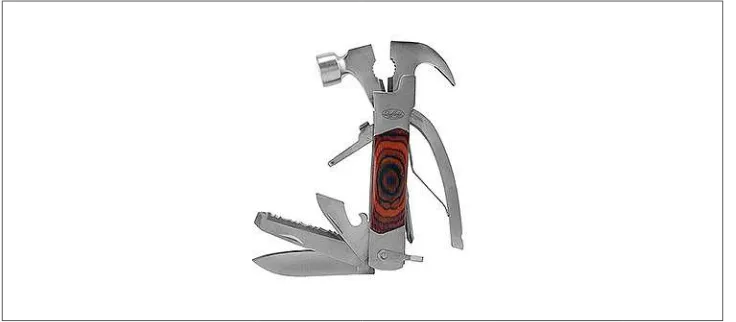
same mentality can be applied to functional programming with pure functions. But the idea is all about simplicity. Have a piece of software do one thing and only one thing. A good example of an SRP violation is a multi-tool (Figure 1-1). They do just about everything but unfortunately are only useful in a pinch.
Figure 1-1. A multi-tool like this has too many responsibilities
Open/Closed Principle
The OCP, sometimes also called encapsulation, is the principle that objects should be open for extending but not for modification. This can be shown in the case of a counter object that has an internal count associated with it. The object has the meth‐ ods increment and decrement. This object should not allow anybody to change the internal count unless it follows the defined API, but it can be extended (e.g., to notify someone of a count change by an object like Notifier).
Liskov Substitution Principle
The LSP states that any subtype should be easily substituted out from underneath a object tree without side effect. For instance, a model car could be substituted for a real car.
Interface Segregation Principle
The ISP is the principle that having many client-specific interfaces is better than a general interface for all clients. This principle is about simplifying the interchange of data between entities. A good example would be separating garbage, compost, and recycling. Instead of having one big garbage can it has three, specific to the garbage type.
1Robert Martin, “The Dependency Inversion Principle,” http://bit.ly/the-DIP.
2Atul Gawande, The Checklist Manifesto (New York: Metropolitan Books), p. 161.
Dependency Inversion Principle
The DIP is a principle that guides us to depend on abstractions, not concretions. What this is saying is that we should build a layer or inheritance tree of objects. The example Robert Martin explains in his original paper1 is that we should have a Key boardReader inherit from a general Reader object instead of being everything in one class. This also aligns well with what Arthur Riel said in Object Oriented Design Heu‐ ristics about avoiding god classes. While you could solder a wire directly from a guitar to an amplifier, it most likely would be inefficient and not sound very good.
The SOLID framework has stood the test of time and has shown up in many books by Martin and Feathers, as well as appearing in Sandi Metz’s book Practical Object-Oriented Design in Ruby. This framework is meant to be a guideline but also to remind us of the simple things so that when we’re writing code we write the best we can. These guidelines help write architectually correct software.
Testing or TDD
In the early days of aviation, pilots didn’t use checklists to test whether their airplane was ready for takeoff. In the book The Right Stuff by Tom Wolfe, most of the original test pilots like Chuck Yeager would go by feel and their own ability to manage the complexities of the craft. This also led to a quarter of test pilots being killed in action.2 Today, things are different. Before taking off, pilots go through a set of checks. Some of these checks can seem arduous, like introducing yourself by name to the other crewmembers. But imagine if you find yourself in a tailspin and need to notify some‐ one of a problem immediately. If you didn’t know their name it’d be hard to commu‐ nicate.
The same is true for good software. Having a set of systematic checks, running regu‐ larly, to test whether our software is working properly or not is what makes software operate consistently.
In the early days of software, most tests were done after writing the original software (see also the waterfall model, used by NASA and other organizations to design soft‐ ware and test it for production). This worked well with the style of project manage‐ ment common then. Similar to how airplanes are still built, software used to be designed first, written according to specs, and then tested before delivery to the cus‐ tomer. But because technology has a short shelf life, this method of testing could take
3Nachiappan Nagappan et al., “Realizing Quality Improvement through Test Driven Development: Results and Experience of Four Industrial Teams,” Empirical Software Engineering 13, no. 3 (2008): 289–302, http://bit.ly/ Nagappanetal.
months or even years. This led to the Agile Manifesto as well as the culture of testing and TDD, spearheaded by Kent Beck, Ward Cunningham, and many others.
The idea of test-driven development is simple: write a test to record what you want to achieve, test to make sure the test fails first, write the code to fix the test, and then, after it passes, fix your code to fit in with the SOLID guidelines. While many people argue that this adds time to the development cycle, it drastically reduces bug deficien‐ cies in code and improves its stability as it operates in production.3
Airplanes, with their low tolerance for failure, mostly operate the same way. Before a pilot flies the Boeing 787 they have spent X amount of hours in a flight simulator understanding and testing their knowledge of the plane. Before planes take off they are tested, and during the flight they are tested again. Modern software development is very much the same way. We test our knowledge by writing tests before deploying it, as well as when something is deployed (by monitoring).
But this still leaves one problem: the reality that since not everything stays the same, writing a test doesn’t make good code. David Heinemer Hanson, in his viral presenta‐ tion about test-driven damage, has made some very good points about how following TDD and SOLID blindly will yield complicated code. Most of his points have to do with needless complication due to extracting out every piece of code into different classes, or writing code to be testable and not readable. But I would argue that this is where the last factor in writing software right comes in: refactoring.
Refactoring
Refactoring is one of the hardest programming practices to explain to nonprogram‐ mers, who don’t get to see what is underneath the surface. When you fly on a plane you are seeing only 20% of what makes the plane fly. Underneath all of the pieces of aluminum and titanium are intricate electrical systems that power emergency lighting in case anything fails during flight, plumbing, trusses engineered to be light and also sturdy—too much to list here. In many ways explaining what goes into an airplane is like explaining to someone that there’s pipes under the sink below that beautiful faucet.
Refactoring takes the existing structure and makes it better. It’s taking a messy circuit breaker and cleaning it up so that when you look at it, you know exactly what is going on. While airplanes are rigidly designed, software is not. Things change rapidly in software. Many companies are continuously deploying software to a production envi‐
ronment. All of that feature development can sometimes cause a certain amount of technical debt.
Technical debt, also known as design debt or code debt, is a metaphor for poor system design that happens over time with software projects. The debilitating problem of technical debt is that it accrues interest and eventually blocks future feature develop‐ ment.
If you’ve been on a project long enough, you will know the feeling of having fast releases in the beginning only to come to a standstill toward the end. Technical debt in many cases arises through not writing tests or not following the SOLID principles. Having technical debt isn’t a bad thing—sometimes projects need to be pushed out earlier so business can expand—but not paying down debt will eventually accrue enough interest to destroy a project. The way we get over this is by refactoring our code.
By refactoring, we move our code closer to the SOLID guidelines and a TDD code‐ base. It’s cleaning up the existing code and making it easy for new developers to come in and work on the code that exists like so:
1. Follow the SOLID guidelines a. Single Responsibility Principle b. Open/Closed Principle c. Liskov Substitution Principle d. Interface Segregation Principle e. Dependency Inversion Principle
2. Implement TDD (test-driven development/design) 3. Refactor your code to avoid a buildup of technical debt
The real question now is what makes the software right?
Writing the Right Software
Writing the right software is much trickier than writing software right. In his book
Specification by Example, Gojko Adzic determines the best approach to writing soft‐ ware is to craft specifications first, then to work with consumers directly. Only after the specification is complete does one write the code to fit that spec. But this suffers from the problem of practice—sometimes the world isn’t what we think it is. Our ini‐ tial model of what we think is true many times isn’t.
Webvan, for instance, failed miserably at building an online grocery business. They had almost $400 million in investment capital and rapidly built infrastructure to sup‐
port what they thought would be a booming business. Unfortunately they were a flop because of the cost of shipping food and the overestimated market for online grocery buying. By many measures they were a success at writing software and building a business, but the market just wasn’t ready for them and they quickly went bankrupt. Today a lot of the infrastructure they built is used by Amazon.com for AmazonFresh.
In theory, theory and practice are the same. In practice they are not. —Albert Einstein
We are now at the point where theoretically we can write software correctly and it’ll work, but writing the right software is a much fuzzier problem. This is where machine learning really comes in.
Writing the Right Software with Machine Learning
In The Knowledge-Creating Company, Nonaka and Takeuchi outlined what made Jap‐ anese companies so successful in the 1980s. Instead of a top-down approach of solv‐ ing the problem, they would learn over time. Their example of kneading bread and turning that into a breadmaker is a perfect example of iteration and is easily applied to software development.
But we can go further with machine learning.
What Exactly Is Machine Learning?
According to most definitions, machine learning is a collection of algorithms, techni‐ ques, and tricks of the trade that allow machines to learn from data—that is, some‐ thing represented in numerical format (matrices, vectors, etc.).
To understand machine learning better, though, let’s look at how it came into exis‐ tence. In the 1950s extensive research was done on playing checkers. A lot of these models focused on playing the game better and coming up with optimal strategies. You could probably come up with a simple enough program to play checkers today just by working backward from a win, mapping out a decision tree, and optimizing that way.
Yet this was a very narrow and deductive way of reasoning. Effectively the agent had to be programmed. In most of these early programs there was no context or irrational behavior programmed in.
About 30 years later, machine learning started to take off. Many of the same minds started working on problems involving spam filtering, classification, and general data analysis.
The important shift here is a move away from computerized deduction to computer‐ ized induction. Much as Sherlock Holmes did, deduction involves using complex
logic models to come to a conclusion. By contrast, induction involves taking data as being true and trying to fit a model to that data. This shift has created many great advances in finding good-enough solutions to common problems.
The issue with inductive reasoning, though, is that you can only feed the algorithm data that you know about. Quantifying some things is exceptionally difficult. For instance, how could you quantify how cuddly a kitten looks in an image?
In the last 10 years we have been witnessing a renaissance around deep learning, which alleviates that problem. Instead of relying on data coded by humans, algo‐ rithms like autoencoders have been able to find data points we couldn’t quantify before.
This all sounds amazing, but with all this power comes an exceptionally high cost and responsibility.
The High Interest Credit Card Debt of Machine Learning
Recently, in a paper published by Google titled “Machine Learning: The High Interest Credit Card of Technical Debt”, Sculley et al. explained that machine learning projects suffer from the same technical debt issues outlined plus more (Table 1-1). They noted that machine learning projects are inherently complex, have vague boundaries, rely heavily on data dependencies, suffer from system-level spaghetti code, and can radically change due to changes in the outside world. Their argument is that these are specifically related to machine learning projects and for the most part they are.
Instead of going through these issues one by one, I thought it would be more interest‐ ing to tie back to our original discussion of SOLID and TDD as well as refactoring and see how it relates to machine learning code.
Table 1-1. The high interest credit card debt of machine learning
Machine learning problem Manifests as SOLID violation
Entanglement Changing one factor changes everything SRP Hidden feedback loops Having built-in hidden features in model OCP Undeclared consumers/visibility debt ISP Unstable data dependencies Volatile data ISP Underutilized data dependencies Unused dimensions LSP
Correction cascade *
Glue code Writing code that does everything SRP Pipeline jungles Sending data through complex workflow DIP Experimental paths Dead paths that go nowhere DIP Configuration debt Using old configurations for new data *
4H. B. McMahan et al., “Ad Click Prediction: A View from the Trenches.” In The 19th ACM SIGKDD Interna‐ tional Conference on Knowledge Discovery and Data Mining, KDD 2013, Chicago, IL, August 11–14, 2013.
5A. Lavoie et al., “History Dependent Domain Adaptation.” In Domain Adaptation Workshop at NIPS ’11, 2011. Machine learning problem Manifests as SOLID violation
Fixed thresholds in a dynamic world Not being flexible to changes in correlations * Correlations change Modeling correlation over causation ML Specific
SOLID Applied to Machine Learning
SOLID, as you remember, is just a guideline reminding us to follow certain goals when writing object-oriented code. Many machine learning algorithms are inherently not object oriented. They are functional, mathematical, and use lots of statistics, but that doesn’t have to be the case. Instead of thinking of things in purely functional terms, we can strive to use objects around each row vector and matrix of data.
SRP
In machine learning code, one of the biggest challenges for people to realize is that the code and the data are dependent on each other. Without the data the machine learning algorithm is worthless, and without the machine learning algorithm we wouldn’t know what to do with the data. So by definition they are tightly intertwined and coupled. This tightly coupled dependency is probably one of the biggest reasons that machine learning projects fail.
This dependency manifests as two problems in machine learning code: entanglement and glue code. Entanglement is sometimes called the principle of Changing Anything Changes Everything or CACE. The simplest example is probabilities. If you remove one probability from a distribution, then all the rest have to adjust. This is a violation of SRP.
Possible mitigation strategies include isolating models, analyzing dimensional depen‐ dencies,4 and regularization techniques.5 We will return to this problem when we review Bayesian models and probability models.
Glue code is the code that accumulates over time in a coding project. Its purpose is usually to glue two separate pieces together inelegantly. It also tends to be the type of code that tries to solve all problems instead of just one.
Whether machine learning researchers want to admit it or not, many times the actual machine learning algorithms themselves are quite simple. The surrounding code is what makes up the bulk of the project. Depending on what library you use, whether it be GraphLab, MATLAB, scikit-learn, or R, they all have their own implementation of vectors and matrices, which is what machine learning mostly comes down to.
OCP
Recall that the OCP is about opening classes for extension but not modification. One way this manifests in machine learning code is the problem of CACE. This can mani‐ fest in any software project but in machine learning projects it is often seen as hidden feedback loops.
A good example of a hidden feedback loop is predictive policing. Over the last few years, many researchers have shown that machine learning algorithms can be applied to determine where crimes will occur. Preliminary results have shown that these algo‐ rithms work exceptionally well. But unfortunately there is a dark side to them as well. While these algorithms can show where crimes will happen, what will naturally occur is the police will start patrolling those areas more and finding more crimes there, and as a result will self-reinforce the algorithm. This could also be called confirmation bias, or the bias of confirming our preconceived notion, and also has the downside of enforcing systematic discrimination against certain demographics or neighborhoods. While hidden feedback loops are hard to detect, they should be watched for with a keen eye and taken out.
LSP
Not a lot of people talk about the LSP anymore because many programmers are advo‐ cating for composition over inheritance these days. But in the machine learning world, the LSP is violated a lot. Many times we are given data sets that we don’t have all the answers for yet. Sometimes these data sets are thousands of dimensions wide. Running algorithms against those data sets can actually violate the LSP. One common manifestation in machine learning code is underutilized data dependencies. Many times we are given data sets that include thousands of dimensions, which can some‐ times yield pertinent information and sometimes not. Our models might take all dimensions yet use one infrequently. So for instance, in classifying mushrooms as either poisonous or edible, information like odor can be a big indicator while ring number isn’t. The ring number has low granularity and can only be zero, one, or two; thus it really doesn’t add much to our model of classifying mushrooms. So that infor‐ mation could be trimmed out of our model and wouldn’t greatly degrade perfor‐ mance.
You might be thinking why this is related to the LSP, and the reason is if we can use only the smallest set of datapoints (or features), we have built the best model possible. This also aligns well with Ockham’s Razor, which states that the simplest solution is the best one.
ISP
The ISP is the notion that a client-specific interface is better than a general purpose one. In machine learning projects this can often be hard to enforce because of the tight coupling of data to the code. In machine learning code, the ISP is usually viola‐ ted by two types of problems: visibility debt and unstable data.
Take for instance the case where a company has a reporting database that is used to collect information about sales, shipping data, and other pieces of crucial informa‐ tion. This is all managed through some sort of project that gets the data into this database. The customer that this database defines is a machine learning project that takes previous sales data to predict the sales for the future. Then one day during cleanup, someone renames a table that used to be called something very confusing to something much more useful. All hell breaks loose and people are wondering what happened.
What ended up happening is that the machine learning project wasn’t the only con‐ sumer of the data; six Access databases were attached to it, too. The fact that there were that many undeclared consumers is in itself a piece of debt for a machine learn‐ ing project.
This type of debt is called visibility debt and while it mostly doesn’t affect a project’s stability, sometimes, as features are built, at some point it will hold everything back. Data is dependent on the code used to make inductions from it, so building a stable project requires having stable data. Many times this just isn’t the case. Take for instance the price of a stock; in the morning it might be valuable but hours later become worthless.
This ends up violating the ISP because we are looking at the general data stream instead of one specific to the client, which can make portfolio trading algorithms very difficult to build. One common trick is to build some sort of exponential weighting scheme around data; another more important one is to version data streams. This versioned scheme serves as a viable way to limit the volatility of a model’s predictions.
DIP
The Dependency Inversion Principle is about limiting our buildups of data and mak‐ ing code more flexible for future changes. In a machine learning project we see con‐ cretions happen in two specific ways: pipeline jungles and experimental paths.
Pipeline jungles are common in data-driven projects and are almost a form of glue code. This is the amalgamation of data being prepared and moved around. In some cases this code is tying everything together so the model can work with the prepared data. Unfortunately, though, over time these jungles start to grow complicated and unusable.
Machine learning code requires both software and data. They are intertwined and inseparable. Sometimes, then, we have to test things during production. Sometimes tests on our machines give us false hope and we need to experiment with a line of code. Those experimental paths add up over time and end up polluting our work‐ space. The best way of reducing the associated debt is to introduce tombstoning, which is an old technique from C.
Tombstones are a method of marking something as ready to be deleted. If the method is called in production it will log an event to a logfile that can be used to sweep the codebase later.
For those of you who have studied garbage collection you most likely have heard of this method as mark and sweep. Basically you mark an object as ready to be deleted and later sweep marked objects out.
Machine Learning Code Is Complex but Not Impossible
At times, machine learning code can be difficult to write and understand, but it is far from impossible. Remember the flight analogy we began with, and use the SOLID guidelines as your “preflight” checklist for writing successful machine learning code —while complex, it doesn’t have to be complicated.
In the same vein, you can compare machine learning code to flying a spaceship—it’s certainly been done before, but it’s still bleeding edge. With the SOLID checklist model, we can launch our code effectively using TDD and refactoring. In essence, writing successful machine learning code comes down to being disciplined enough to follow the principles of design we’ve laid out in this chapter, and writing tests to sup‐ port your code-based hypotheses. Another critical element in writing effective code is being flexible and adapting to the changes it will encounter in the real world.
TDD: Scientific Method 2.0
Every true scientist is a dreamer and a skeptic. Daring to put a person on the moon was audacious, but through systematic research and development we have accom‐ plished that and much more. The same is true with machine learning code. Some of the applications are fascinating but also hard to pull off.
The secret to doing so is to use the checklist of SOLID for machine learning and the tools of TDD and refactoring to get us there.
TDD is more of a style of problem solving, not a mandate from above. What testing gives us is a feedback loop that we can use to work through tough problems. As scien‐ tists would assert that they need to first hypothesize, test, and theorize, we can assert that as a TDD practitioner, the process of red (the tests fail), green (the tests pass), refactor is just as viable.
This book will delve heavily into applying not only TDD but also SOLID principles to machine learning, with the goal being to refactor our way to building a stable, scala‐ ble, and easy-to-use model.
Refactoring Our Way to Knowledge
As mentioned, refactoring is the ability to edit one’s work and to rethink what was once stated. Throughout the book we will talk about refactoring common machine learning pitfalls as it applies to algorithms.
The Plan for the Book
This book will cover a lot of ground with machine learning, but by the end you should have a better grasp of how to write machine learning code as well as how to deploy to a production environment and operate at scale. Machine learning is a fasci‐ nating field that can achieve much, but without discipline, checklists, and guidelines, many machine learning projects are doomed to fail.
Throughout the book we will tie back to the original principles in this chapter by talking about SOLID principles, testing our code (using various means), and refactor‐ ing as a way to continually learn from and improve the performance of our code. Every chapter will explain the Python packages we will use and describe a general testing plan. While machine learning code isn’t testable in a one-to-one case, it ends up being something for which we can write tests to help our knowledge of the problem.
CHAPTER 2
A Quick Introduction to Machine Learning
You’ve picked up this book because you’re interested in machine learning. While you probably have an idea of what machine learning is, the subject is often defined some‐ what vaguely. In this quick introduction, I’ll go over what exactly machine learning is, and provide a general framework for thinking about machine learning algorithms.
What Is Machine Learning?
Machine learning is the intersection between theoretically sound computer science and practically noisy data. Essentially, it’s about machines making sense out of data in much the same way that humans do.
Machine learning is a type of artificial intelligence whereby an algorithm or method extracts patterns from data. Machine learning solves a few general problems; these are listed in Table 2-1 and described in the subsections that follow.
Table 2-1. The problems that machine learning can solve
Problem Machine learning category
Fitting some data to a function or function approximation Supervised learning Figuring out what the data is without any feedback Unsupervised learning Maximizing rewards over time Reinforcement learning
Supervised Learning
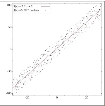
Supervised learning, or function approximation, is simply fitting data to a function of any variety. For instance, given the noisy data shown in Figure 2-1, you can fit a line that generally approximates it.
Figure 2-1. This data fits quite well to a straight line
Unsupervised Learning
Unsupervised learning involves figuring out what makes the data special. For instance, if we were given many data points, we could group them by similarity (Figure 2-2), or perhaps determine which variables are better than others.
Figure 2-2. Two clusters grouped by similarity
Reinforcement Learning
Reinforcement learning involves figuring out how to play a multistage game with rewards and payoffs. Think of it as the algorithms that optimize the life of something. A common example of a reinforcement learning algorithm is a mouse trying to find cheese in a maze. For the most part, the mouse gets zero reward until it finally finds the cheese.
We will discuss supervised and unsupervised learning in this book but skip reinforce‐ ment learning. In the final chapter, I include some resources that you can check out if you’d like to learn more about reinforcement learning.
What Can Machine Learning Accomplish?
What makes machine learning unique is its ability to optimally figure things out. But each machine learning algorithm has quirks and trade-offs. Some do better than oth‐ ers. This book covers quite a few algorithms, so Table 2-2 provides a matrix to help you navigate them and determine how useful each will be to you.
Table 2-2. Machine learning algorithm matrix
Algorithm Learning type Class Restriction bias Preference bias
K-Nearest Neighbors
Supervised Instance based Generally speaking, KNN is good for measuring distance-based approximations; it suffers from the curse of dimensionality
Prefers problems that are distance based
Naive Bayes Supervised Probabilistic Works on problems where the inputs are independent from each other
Prefers problems where the probability will always be greater than zero for each class
Algorithm Learning type Class Restriction bias Preference bias
Decision Trees/ Random Forests
Supervised Tree Becomes less useful on problems with low covariance
Clustering Unsupervised Clustering No restriction Prefers data that is in groupings given some form of
Must be a nondegenerate matrix Will work much better on matricies that don’t have inversion issues
Bagging Meta-heuristic Meta-heuristic Will work on just about anything Prefers data that isn’t highly variable
Refer to this matrix throughout the book to understand how these algorithms relate to one another.
Machine learning is only as good as what it applies to, so let’s get to implementing some of these algorithms! Before we get started, you will need to install Python, which you can do at https://www.python.org/downloads/. This book was tested using Python 2.7.12, but most likely it will work with Python 3.x as well. All of those changes will be annotated in the book’s coding resources, which are available on Git‐ Hub.
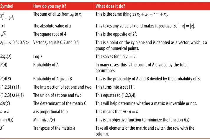
Mathematical Notation Used Throughout the Book
This book uses mathematics to solve problems, but all of the examples are programmer-centric. Throughout the book, I’ll use the mathematical notations shown in Table 2-3.
Table 2-3. Mathematical notations used in this book’s examples
Symbol How do you say it? What does it do?
∑in= 0xi The sum of all xs from x0 to xn This is the same thing as x0 + x1 + ⋯ + xn.
ǀxǀ The absolute value of x This takes any value of x and makes it positive. So |–x| = |x|. 4 The square root of 4 This is the opposite of 22.
zk = < 0.5, 0.5 > Vector zk equals 0.5 and 0.5 This is a point on the xy plane and is denoted as a vector, which is a
group of numerical points.
log2(2) Log 2 This solves for i in 2i = 2.
P(A) Probability of A In many cases, this is the count of A divided by the total occurrences.
P(AǀB) Probability of A given B This is the probability of A and B divided by the probability of B. {1,2,3} ∩ {1} The intersection of set one and two This turns into a set {1}.
{1,2,3} ∪ {4,1} The union of set one and two This equates to {1,2,3,4}.
det(C) The determinant of the matrix C This will help determine whether a matrix is invertible or not.
a∝b a is proportional to b This means that m · a = b.
min f(x) Minimize f(x) This is an objective function to minimize the function f(x).
XT Transpose of the matrix X Take all elements of the matrix and switch the row with the
column.
Conclusion
This isn’t an exhaustive introduction to machine learning, but that’s okay. There’s always going to be a lot for us all to learn when it comes to this complex subject, but for the remainder of this book, this should serve us well in approaching these problems.
CHAPTER 3
K-Nearest Neighbors
Have you ever bought a house before? If you’re like a lot of people around the world, the joy of owning your own home is exciting, but the process of finding and buying a house can be stressful. Whether we’re in a economic boom or recession, everybody wants to get the best house for the most reasonable price.
But how would you go about buying a house? How do you appraise a house? How does a company like Zillow come up with their Zestimates? We’ll spend most of this chapter answering questions related to this fundamental concept: distance-based approximations.
First we’ll talk about how we can estimate a house’s value. Then we’ll discuss how to classify houses into categories such as “Buy,” “Hold,” and “Sell.” At that point we’ll talk about a general algorithm, K-Nearest Neighbors, and how it can be used to solve problems such as this. We’ll break it down into a few sections of what makes some‐ thing near, as well as what a neighborhood really is (i.e., what is the optimal K for something?).
How Do You Determine Whether You Want to Buy a
House?
This question has plagued many of us for a long time. If you are going out to buy a house, or calculating whether it’s better to rent, you are most likely trying to answer this question implicitly. Home appraisals are a tricky subject, and are notorious for drift with calculations. For instance on Zillow’s website they explain that their famous Zestimate is flawed. They state that based on where you are looking, the value might drift by a localized amount.
Location is really key with houses. Seattle might have a different demand curve than San Francisco, which makes complete sense if you know housing! The question of whether to buy or not comes down to value amortized over the course of how long you’re living there. But how do you come up with a value?
How Valuable Is That House?
Things are worth as much as someone is willing to pay. —Old Saying
Valuing a house is tough business. Even if we were able to come up with a model with many endogenous variables that make a huge difference, it doesn’t cover up the fact that buying a house is subjec‐ tive and sometimes includes a bidding war. These are almost impossible to predict. You’re more than welcome to use this to value houses, but there will be errors that take years of experience to overcome.
A house is worth as much as it’ll sell for. The answer to how valuable a house is, at its core, is simple but difficult to estimate. Due to inelastic supply, or because houses are all fairly unique, home sale prices have a tendency to be erratic. Sometimes you just love a house and will pay a premium for it.
But let’s just say that the house is worth what someone will pay for it. This is a func‐ tion based on a bag of attributes associated with houses. We might determine that a good approach to estimating house values would be:
Equation 3-1. House value
HouseValue= f Space,LandSize,Rooms,Bathrooms,⋯
This model could be found through regression (which we’ll cover in Chapter 5) or other approximation algorithms, but this is missing a major component of real estate: “Location, Location, Location!” To overcome this, we can come up with something called a hedonic regression.
Hedonic Regression
You probably already know of a frequently used real-life hedonic regression: the CPI index. This is used as a way of decomposing baskets of items that people commonly buy to come up with an index for inflation.
Economics is a dismal science because we’re trying to approximate rational behaviors. Unfortunately we are predictably irrational (shout-out to Dan Ariely). But a good algorithm for valuing houses that is similar to what home appraisers use is called hedonic regression.
The general idea with hard-to-value items like houses that don’t have a highly liquid market and suffer from subjectivity is that there are externalities that we can’t directly estimate. For instance, how would you estimate pollution, noise, or neighbors who are jerks?
To overcome this, hedonic regression takes a different approach than general regres‐ sion. Instead of focusing on fitting a curve to a bag of attributes, it focuses on the components of a house. For instance, the hedonic method allows you to find out how much a bedroom costs (on average).
Take a look at the Table 3-1, which compares housing prices with number of bed‐ rooms. From here we can fit a naive approximation of value to bedroom number, to come up with an estimate of cost per bedroom.
Table 3-1. House price by number of bedrooms
Price (in $1,000) Bedrooms
$899 4
$399 3
$749 3
$649 3
This is extremely useful for valuing houses because as consumers, we can use this to focus on what matters to us and decompose houses into whether they’re overpriced because of bedroom numbers or the fact that they’re right next to a park.
This gets us to the next improvement, which is location. Even with hedonic regres‐ sion, we suffer from the problem of location. A bedroom in SoHo in London, Eng‐ land is probably more expensive than a bedroom in Mumbai, India. So for that we need to focus on the neighborhood.
What Is a Neighborhood?
The value of a house is often determined by its neighborhood. For instance, in Seattle, an apartment in Capitol Hill is more expensive than one in Lake City. Generally
1Van Ommeren et al., “Estimating the Marginal Willingness to Pay for Commuting,” Journal of Regional Sci‐ ence 40 (2000): 541–63.
speaking, the cost of commuting is worth half of your hourly wage plus maintenance and gas,1 so a neighborhood closer to the economic center is more valuable.
But how would we focus only on the neighborhood?
Theoretically we could come up with an elegant solution using something like an exponential decay function that weights houses closer to downtown higher and far‐ ther houses lower. Or we could come up with something static that works exception‐ ally well: K-Nearest Neighbors.
K-Nearest Neighbors
What if we were to come up with a solution that is inelegant but works just as well? Say we were to assert that we will only look at an arbitrary amount of houses near to a similar house we’re looking at. Would that also work?
Surprisingly, yes. This is the K-Nearest Neighbor (KNN) solution, which performs exceptionally well. It takes two forms: a regression, where we want a value, or a classi‐ fication. To apply KNN to our problem of house values, we would just have to find the nearest K neighbors.
The KNN algorithm was originally introduced by Drs. Evelyn Fix and J. L. Hodges Jr, in an unpublished technical report written for the U.S. Air Force School of Aviation Medicine. Fix and Hodges’ original research focused on splitting up classification problems into a few subproblems:
• Distributions F and G are completely known.
• Distributions F and G are completely known except for a few parameters. • F and G are unknown, except possibly for the existence of densities.
Fix and Hodges pointed out that if you know the distributions of two classifications or you know the distribution minus some parameters, you can easily back out useful solutions. Therefore, they focused their work on the more difficult case of finding classifications among distributions that are unknown. What they came up with laid the groundwork for the KNN algorithm.
This opens a few more questions:
• What are neighbors, and what makes them near? • How do we pick the arbitrary number of neighbors, K?
• What do we do with the neighbors afterward?
Mr. K’s Nearest Neighborhood
We all implicitly know what a neighborhood is. Whether you live in the woods or a row of brownstones, we all live in a neighborhood of sorts. A neighborhood for lack of a better definition could just be called a cluster of houses (we’ll get to clustering later).
A cluster at this point could be just thought of as a tight grouping of houses or items in n dimensions. But what denotes a “tight grouping”? Since you’ve most likely taken a geometry class at some time in your life, you’re probably thinking of the Pythagor‐ ean theorem or something similar, but things aren’t quite that simple. Distances are a class of functions that can be much more complex.
Distances
As the crow flies.—Old Saying
Geometry class taught us that if you sum the square of two sides of a triangle and take its square root, you’ll have the side of the hypotenuse or the third side (Figure 3-1). This as we all know is the Pythagorean theorem, but distances can be much more complicated. Distances can take many different forms but generally there are geomet‐ rical, computational, and statistical distances which we’ll discuss in this section.
Figure 3-1. Pythagorean theorem
Triangle Inequality
One interesting aspect about the triangle in Figure 3-1 is that the length of the hypo‐ tenuse is always less than the length of each side added up individually (Figure 3-2).
Figure 3-2. Triangle broken into three line segments
Stated mathematically: ∥x∥ + ∥y∥ ≤ ∥x∥ + ∥y∥. This inequality is important for find‐ ing a distance function; if the triangle inequality didn’t hold, what would happen is distances would become slightly distorted as you measure distance between points in a Euclidean space.
Geometrical Distance
The most intuitive distance functions are geometrical. Intuitively we can measure how far something is from one point to another. We already know about the Pytha‐ gorean theorem, but there are an infinite amount of possibilities that satisfy the trian‐ gle inequality.
Stated mathematically we can take the Pythagorean theorem and build what is called the Euclidean distance, which is denoted as:
d x,y = ∑in= 0 x i−yi 2
As you can see, this is similar to the Pythagorean theorem, except it includes a sum. Mathematics gives us even greater ability to build distances by using something called a Minkowski distance (see Figure 3-3):
dpx,y = ∑in= 0x i−yi p
1 p
This p can be any integer and still satisfy the triangle inequality.
Figure 3-3. Minkowski distances as n increases (Source: Wikimedia)
Cosine similarity
One last geometrical distance is called cosine similarity or cosine distance. The beauty of this distance is its sheer speed at calculating distances between sparse vec‐ tors. For instance if we had 1,000 attributes collected about houses and 300 of these were mutually exclusive (meaning that one house had them but the others don’t), then we would only need to include 700 dimensions in the calculation.
Visually this measures the inner product space between two vectors and presents us with cosine as a measure. Its function is:
d x,y = ∥xx∥ ∥·yy∥
where ∥x∥ denotes the Euclidean distance discussed earlier.
Geometrical distances are generally what we want. When we talk about houses we want a geometrical distance. But there are other spaces that are just as valuable: com‐ putational, or discrete, as well as statistical distances.
Computational Distances
Imagine you want to measure how far it is from one part of the city to another. One way of doing this would be to utilize coordinates (longitude, latitude) and calculate a Euclidean distance. Let’s say you’re at Saint Edward State Park in Kenmore, WA (47.7329290, -122.2571466) and you want to meet someone at Vivace Espresso on Capitol Hill, Seattle, WA (47.6216650, -122.3213002).
Using the Euclidean distance we would calculate:
47 . 73 − 47 . 622+ − 122 . 26 + 122 . 322≈ 0 . 13
This is obviously a small result as it’s in degrees of latitude and longitude. To convert this into miles we would multiply it by 69.055, which yields approximately 8.9 miles (14.32 kilometers). Unfortunately this is way off! The actual distance is 14.2 miles (22.9 kilometers). Why are things so far off?
Note that 69.055 is actually an approximation of latitude degrees to miles. Earth is an ellipsoid and therefore calculating distances actually depends on where you are in the world. But for such a short distance it’s good enough.
If I had the ability to lift off from Saint Edward State Park and fly to Vivace then, yes, it’d be shorter, but if I were to walk or drive I’d have to drive around Lake Washington (see Figure 3-4).
This gets us to the motivation behind computational distances. If you were to drive from Saint Edward State Park to Vivace then you’d have to follow the constraints of a road.
Figure 3-4. Driving to Vivace from Saint Edward State Park
Manhattan distance
This gets us into what is called the Taxicab distance or Manhattan distance.
Equation 3-2. Manhattan distance
∑in= 0 x i−yi
Note that there is no ability to travel out of bounds. So imagine that your metric space is a grid of graphing paper and you are only allowed to draw along the boxes.
The Manhattan distance can be used for problems such as traversal of a graph and discrete optimization problems where you are constrained by edges. With our hous‐ ing example, most likely you would want to measure the value of houses that are close by driving, not by flying. Otherwise you might include houses in your search that are across a barrier like a lake, or a mountain!
Levenshtein distance
Another distance that is commonly used in natural language processing is the Lev‐ enshtein distance. An analogy of how Levenshtein distance works is by changing one neighborhood to make an exact copy of another. The number of steps to make that happen is the distance. Usually this is applied with strings of characters to determine how many deletions, additions, or substitutions the strings require to be equal. This can be quite useful for determining how similar neighborhoods are as well as strings. The formula for this is a bit more complicated as it is a recursive function, so instead of looking at the math we’ll just write Python for this:
def lev(a, b):
if not a: return len(b) if not b: return len(a)
return min(lev(a[1:], b[1:])+(a[0] != b[0]), lev(a[1:], b)+1, lev(a, b[1:])+1) This is an extremely slow algorithm and I’m only putting it here for understanding, not to actually implement. If you’d like to imple‐ ment Levenshtein, you will need to use dynamic programming to have good performance.
Statistical Distances
Last, there’s a third class of distances that I call statistical distances. In statistics we’re taught that to measure volatility or variance, we take pairs of datapoints and measure the squared difference. This gives us an idea of how dispersed the population is. This can actually be used when calculating distance as well, using what is called the Maha‐ lanobis distance.
Imagine for a minute that you want to measure distance in an affluent neighborhood that is right on the water. People love living on the water and the closer you are to it, the higher the home value. But with our distances discussed earlier, whether compu‐ tational or geometrical, we would have a bad approximation of this particular neigh‐ borhood because those distance calculations are primarily spherical in nature (Figures 3-5 and 3-6).
Figure 3-5. Driving from point A to point B on a city block
Figure 3-6. Straight line between A and B
This seems like a bad approach for this neighborhood because it is not spherical in nature. If we were to use Euclidean distances we’d be measuring values of houses not on the beach. If we were to use Manhattan distances we’d only look at houses close by the road.
Mahalanobis distance
Another approach is using the Mahalanobis distance. This takes into consideration some other statistical factors:
d x,y = ∑in= 1 xi−yi 2
si2
What this effectively does is give more stretch to the grouping of items (Figure 3-7):
Figure 3-7. Mahalanobis distance
Jaccard distance
Yet another distance metric is called the Jaccard distance. This takes into considera‐ tion the population of overlap. For instance, if the number of attributes for one house match another, then they would be overlapping and therefore close in distance, whereas if the houses had diverging attributes they wouldn’t match. This is primarily used to quickly determine how similar text is by counting up the frequencies of letters in a string and then counting the characters that are not the same across both. Its for‐ mula is:
J X,Y = XX∩∪YY
This finishes up a primer on distances. Now that we know how to measure what is close and what is far, how do we go about building a grouping or neighborhood? How many houses should be in the neighborhood?
Curse of Dimensionality
Before we continue, there’s a serious concern with using distances for anything and that is called the curse of dimensionality. When we model high-dimension spaces, our approximations of distance become less reliable. In practice it is important to realize that finding features of data sets is essential to making a resilient model. We will talk about feature engineering in Chapter 10 but for now be cognizant of the problem. Figure 3-8 shows a visual way of thinking about this.
Figure 3-8. Curse of dimensionality
As Figure 3-8 shows, when we put random dots on a unit sphere and measure the distance from the origin (0,0,0), we find that the distance is always 1. But if we were to project that onto a 2D space, the distance would be less than or equal to 1. This same truth holds when we expand the dimensions. For instance, if we expanded our set from 3 dimensions to 4, it would be greater than or equal to 1. This inability to center in on a consistent distance is what breaks distance-based models, because all of the data points become chaotic and move away from one another.
How Do We Pick K?
Picking the number of houses to put into this model is a difficult problem—easy to verify but hard to calculate beforehand. At this point we know how we want to group things, but just don’t know how many items to put into our neighborhood. There are a few approaches to determining an optimal K, each with their own set of downsides:
• Guessing • Using a heuristic
• Optimizing using an algorithm
Guessing K
Guessing is always a good solution. Many times when we are approaching a problem, we have domain knowledge of it. Whether we are an expert or not, we know about the problem enough to know what a neighborhood is. My neighborhood where I live, for instance, is roughly 12 houses. If I wanted to expand I could set my K to 30 for a more flattened-out approximation.
Heuristics for Picking K
There are three heuristics that can help you determine an optimal K for a KNN algorithm:
1. Use coprime class and K combinations
2. Choose a K that is greater or equal to the number of classes plus one 3. Choose a K that is low enough to avoid noise
Use coprime class and K combinations
Picking coprime numbers of classes and K will ensure fewer ties. Coprime numbers are two numbers that don’t share any common divisors except for 1. So, for instance, 4 and 9 are coprime while 3 and 9 are not. Imagine you have two classes, good and bad. If we were to pick a K of 6, which is even, then we might end up having ties. Graphically it looks like Figure 3-9.
Figure 3-9. Tie with K=6 and two classes
If you picked a K of 5 instead (Figure 3-10), there wouldn’t be a tie.
Figure 3-10. K=5 with two classes and no tie
Choose a K that is greater or equal to the number of classes plus one
Imagine there are three classes: lawful, chaotic, and neutral. A good heuristic is to pick a K of at least 3 because anything less will mean that there is no chance that each class will be represented. To illustrate, Figure 3-11 shows the case of K=2.
Figure 3-11. With K=2 there is no possibility that all three classes will be represented
Note how there are only two classes that get the chance to be used. Again, this is why we need to use at least K=3. But based on what we found in the first heuristic, ties are not a good thing. So, really, instead of K=3, we should use K=4 (as shown in Figure 3-12).
Figure 3-12. With K set greater than the number of classes, there is a chance for all classes to be represented
Choose a K that is low enough to avoid noise
As K increases, you eventually approach the size of the entire data set. If you were to pick the entire data set, you would select the most common class. A simple example is mapping a customer’s affinity to a brand. Say you have 100 orders as shown in Table 3-2.
Table 3-2. Brand to count
If we were to set K=100, our answer will always be Ion 5 because Ion 5 is the distribu‐ tion (the most common class) of the order history. That is not really what we want; instead, we want to determine the most recent order affinity. More specifically, we want to minimize the amount of noise that comes into our classification. Without coming up with a specific algorithm for this, we can justify K being set to a much lower rate, like K=3 or K=11.
Algorithms for picking K
Picking K can be somewhat qualitative and nonscientific, and that’s why there are many algorithms showing how to optimize K over a given training set. There are many approaches to choosing K, ranging from genetic algorithms to brute force to grid searches. Many people assert that you should determine K based on domain knowledge that you have as the implementor. For instance, if you know that 5 is good enough, you can pick that. This problem where you are trying to minimize error based on an arbitrary K is known as a hill climbing problem. The idea is to iterate through a couple of possible Ks until you find a suitable error. The difficult part about finding a K using an approach like genetic algorithms or brute force is that as K increases, the complexity of the classification also increases and slows down perfor‐ mance. In other words, as you increase K, the program actually gets slower. If you want to learn more about genetic algorithms applied to finding an optimal K, you can read more about it in Nigsch et al.’s Journal of Chemical Information and Modeling
article, “Melting Point Prediction Employing k-Nearest Neighbor Algorithms and Genetic Parameter Optimization.” Personally, I think iterating twice through 1% of the population size is good enough. You should have a decent idea of what works and what doesn’t just by experimenting with different Ks.
Valuing Houses in Seattle
Valuing houses in Seattle is a tough gamble. According to Zillow, their Zestimate is consistently off in Seattle. Regardless, how would we go about building something that tells us how valuable the houses are in Seattle? This section will walk through a simple example so that you can figure out with reasonable accuracy what a house is worth based on freely available data from the King County Assessor.
If you’d like to follow along in the code examples, check out the GitHub repo.
About the Data
While the data is freely available, it wasn’t easy to put together. I did a bit of cajoling to get the data well formed. There’s a lot of features, ranging from inadequate parking to whether the house has a view of Mount Rainier or not. I felt that while that was an interesting exercise, it’s not really important to discuss here. In addition to the data they gave us, geolocation has been added to all of the datapoints so we can come up with a location distance much easier.
General Strategy
Our general strategy for finding the values of houses in Seattle is to come up with something we’re trying to minimize/maximize so we know how good the model is. Since we will be looking at house values explicitly, we can’t calculate an “Accuracy” rate because every value will be different. So instead we will utilize a different metric called mean absolute error.
With all models, our goal is to minimize or maximize something, and in this case we’re going to minimize the mean absolute error. This is defined as the average of the absolute errors. The reason we’ll use absolute error over any other common metrics (like mean squared error) is that it’s useful. When it comes to house values it’s hard to get intuition around the average squared error, but by using absolute error we can instead say that our model is off by $70,000 or similar on average.
As for unit testing and functional testing, we will approach this in a random fashion by stratifying the data into multiple chunks so that we can sample the mean absolute errors. This is mainly so that we don’t find just one weird case where the mean abso‐ lute error was exceptionally low. We will not be talking extensively here about unit testing because this is an early chapter and I feel that it’s more important to focus on the overall testing of the model through mean absolute error.
Coding and Testing Design
The basic design of the code for this chapter is going to center around a Regressor class. This class will take in King County housing data that comes in via a flat, calcu‐ late an error rate, and do the regression (Figure 3-13). We will not be doing any unit testing in this chapter but instead will visually test the code using the plot_error function we will build inside of the Regressor class.