Extending the New Keynesian Monetary
Model with Data Revision Processes
?Jesús Vázquez,1 Ramón María-Dolores2 and Juan M. Londoño1
1
Universidad del País Vasco
2
Universidad de Murcia
Abstract. This paper proposes an extended version of the New Key-nesian Monetary (NKM) model which contemplates revision processes of output and inflation data in order to assess the importance of data revisions on the estimated monetary policy rule parameters. The estima-tion results of the extended NKM model suggest that real-time data are not rational forecasts of revised data. These results are in line with the evidence provided by Aruoba (2008) using a reduced-form econometric approach. Moreover, the different policy parameter estimates obtained depending on whether or not the revision processes are assumed to be well behaved, provide evidence that policymakers decisions could be de-termined by the availability of data at the time of policy implementation. Key words: NKM model, monetary policy rule, indirect inference, real-time data, (non-)rational forecast errors
JEL classification numbers: C32, E30, E52
1
INTRODUCTION
Nowadays, the importance of timing and availability of the data used in the empirical evaluation of policy rules has converted into some-thing crucial. Some preliminary studies about real-time data such as those of Maravall and Pierce (1986), Trivellato and Rettore (1986) and Ghyssels, Swanson and Callan (2002) have examined revision process errors. Maravall and Pierce (1986) analyze how preliminary and incomplete data affect monetary policy and demonstrate that, even though revisions to measures of money supply are large, mon-etary policy would not have been much different if more accurate data had been known. By contrast, Ghyssels, Swanson and Callan (2002)find that a Taylor-type rule would have been significantly im-proved if policymakers had waited for data to be revised rather than reacting to newly released data.3
Two of the most well-known studies that compare results based on real-time data with those obtained with revised data are Diebold and Rudebusch (1991) and Orphanides (2001). The former shows that the index of leading indicators does a much worse job in predict-ing future movements of output in real time than it does after data are revised. The latter examines parameter as well as model specifi -cation uncertainty in the Taylor-rule by using data over a period of more than 20 years. The paper concludes that the Taylor principle does not prevail using real-time data. This empirical evidence is in sharp contrast with that found by Clarida, Galí and Gertler (2000). With regard to Taylor-rule parameters, Rudebusch (2002) indicates that data uncertainty potentially plays an important role in reduc-ing the coefficients of the rule that characterize both policy inertia and shock persistence.4 The main advantage of using real-time data
in estimating policy rules is to reduce the effects of parameter un-certainty in actual policy setting since the researcher can estimate
3
Mankiw, Runkle and Shapiro (1984) is a seminal paper in this branch of litera-ture. They develop a theoretical framework for analyzing initial announcements of economic data and apply that framework to the money stock.
4 By using reduced-form estimation approaches, some empirical studies, such as
policy rules with data which were truly available at any given point in time. This is particularly important with seasonally adjusted data as such data are subject to revisions based on two-sidedfilters.5
As pointed out by Aruoba (2008), should revisions of real-time data be rational forecast errors, then the arrival of revised data would not be relevant for policy makers’ decisions and policy rule estimates would be rather similar using either revised or real-time data. More-over, Aruoba (2008) documents the empirical properties of revisions to major macroeconomic variables in the U.S. and points out that they are not well-behaved. That is, they do not satisfy simple desir-able properties such as zero mean, which indicates that the revisions of initial announcements made by statistical agencies are biased, and that they might be predictable using the information set available at the time of the initial announcement.
The literature estimating policy rules with real-time data cited above uses reduced-form econometric approaches. This paper ex-tends the NKM model to include revision processes of output and inflation data, and thus to analyze revised and real-time data to-gether by using a structural econometric approach. This extension allows for (i) a joint estimation procedure of both monetary policy rule and revision process parameters, (ii) an assessment of the inter-action between these two sets of parameters and, (iii) a test of the null hypothesis establishing that real-time data are a rational fore-cast of revised data in the context of a dynamic structural general equilibrium (DSGE) model.
The use of real-time data in the estimation of a DSGE model may look tricky because private agents’ (households andfirms) deci-sions determine the true (revised) values of macroeconomic variables, such as output and inflation, and they are not observable without error by policymakers in real time. The problem is easily solved by augmenting the NKM model with the revision processes of output and inflation. In particular, these revision processes are allowed to
5 Kavajecz and Collins (1995) conclude, using Monte Carlo simulations, that
be determined by the information available at the time the initial announcements of output and inflation are released.
We follow a classical approach based on the indirect inference principle suggested by Smith (1993, 2008) to estimate our extended version of the NKM model. In particular, we follow Smith (1993) by using an unrestricted VAR as the auxiliary model. More precisely, the distance function is built upon the coefficients estimated from a five-variable VAR that considers U.S. quarterly data of revised output growth, revised inflation, real-time output growth, real-time inflation and the Fed funds rate.
The estimation results show that most policy rule parameter esti-mates depend to an important extent on whether or not the revision processes of output and inflation are assumed to be well-behaved. In particular, the estimates of policy inertia and output gap pa-rameters are larger whereas monetary shock persistence substan-tially decreases by allowing for the possibility of non-rational revision processes. These differences provide empirical evidence that policy-makers’ decisions could be determined by the availability of data at the time of policy implementation. Moreover, the estimates of the revision process parameters show that the initial announcements of output and inflation are not rational forecasts. For instance, a 1% increase in the initial announcement of inflation leads to a downward revision in output of 2.96%. These estimation results are in line with the empirical evidence provided by Aruoba (2008) mentioned above, who finds that data revisions are not well-behaved (i.e. they are not white noise processes).
2
AN NKM MODEL AUGMENTED WITH
DATA REVISION PROCESSES
The model analyzed in this paper is a standard NKM model aug-mented with data revision processes. It is given by the following set of equations:
xt=Etxt+1−τ(it−Etπt+1)−φ(1−ρχ)χt, (1)
πt=βEtπt+1+κxt+zt, (2)
it =ρit−1+ (1−ρ)[ψ1πrt−1+ψ2xrt−1] +vt. (3)
xt≡xrt +rxt, (4)
πt≡πrt +rtπ, (5)
rxt =bxxxrt +bxππrt + rxt, (6)
rπt =bπxxrt +bπππrt + rπt, (7)
where x denotes revised output gap (that is, the log-deviation of output with respect to the level of output underflexible prices) andπ
andidenote the deviations from the steady states of revised inflation and nominal interest rate, respectively. πr
t andxrt are real-time data
for inflation and output gap, respectively.Etdenotes the conditional
expectation based on the agents’ information set at timet. χ,z and
v denote aggregate productivity, cost-push inflation and monetary policy shocks, respectively. Each of these shocks is further assumed to follow a first-order autoregressive process:
χt=ρχχt−1+ χt, (8)
zt =ρzzt−1+ zt, (9)
vt =ρvvt−1+ vt, (10)
where χt, zt and vt denote i.i.d. random innovations associated
with these shocks and their standard deviations are denoted by σχ,
σz andσv, respectively.
parameter τ > 0 represents the intertemporal elasticity of substi-tution obtained when assuming a standard constant relative risk aversion utility function.
Equation (2) is the New Phillips curve that is obtained in a sticky price à la Calvo (1983) model where monopolistically competitive
firms produce (a continuum of) differentiated goods and each firm faces a downward sloping demand curve for its produced good. The parameter β ∈ (0,1) is the agent discount factor, and κ measures the slope of the New Phillips curve that is related to other structural parameters as follows
κ= [(1/τ) +η](1−ω)(1−ωβ)
ω .
In particular, κ is a decreasing function of Calvo’s probability, ω. The parameter ω is a measure of the degree of nominal rigidity; a largerωimplies that fewerfirms adjust prices in each period and that the expected time between price changes is longer.6 At this point, it
is worthwhile emphasizing that the IS and Phillips curve equations are described in terms of the revised output and inflation data since they are indeed determined by the optimal choices of private agents (households and firms).
In contrast to Equation (1)-(2), Equation (3) describes the mon-etary policy rule based on real-time data of output and inflation truly available at the time of implementing monetary policy. More-over, the nominal interest rate exhibits smoothing behaviour. As pointed out by Aruoba (2008), the initial announcement of quar-terly (monthly) macroeconomic variables corresponding to a par-ticular quarter (month) appears in the vintage of the next quarter (month), roughly 45 (at least 15) days after the end of the quarter (month). Then, a backward-looking Taylor rule as (3), that includes lagged values of real-time data on output and inflation, would more accurately approximate the information set available to the Fed at the time of implementing the policy7.
6 See, for instance, Walsh (2003, chapter 5.4) for a detailed analytical derivation of
the New Phillips curve.
7 Notice that a backward-looking policy rule does not necessarily exclude the
ex-The NKM model is extended to incorporate the revision processes of output and inflation data, respectively. Equations (4) and (5) are identities showing how revised data of output and inflation are re-lated to real-time output and inflation, respectively. Then, rx
t (rtπ)
denotes the revision of output (inflation).8 Equations (6) and (7)
describe the revision processes associated with output and inflation, respectively. These processes allow for the existence of non-zero cor-relations between output and inflation revisions and the initial an-nouncements of these variables.9 r
xt and rπt denote i.i.d. random
innovations associated with the revision processes where the corre-sponding standard deviations are denoted byσr
xandσrπ, respectively.
Finally, the model is completed by the following identities:
xt =Et−1xt+ (xt−Et−1xt),
πt=Et−1πt+ (πt−Et−1πt).
The system of equations (1)-(10) (together with the latter two identities involving forecast errors) can be written in matrix form as follows:
Γ0Yt =Γ1Yt−1+Ψ t+Πηt, (11)
Yt= (xt, πt, it, Etxt+1, Etπt+1, χt, zt, vt, xrt, πrt, rxt, rπt)0,
t = ( χt, zt, vt, rxt, rπt)0.
ηt= (xt−Et−1xt, πt−Et−1πt)0.
Equation (11) represents a linear rational expectations (LRE) system. It is well known that LRE systems deliver multiple sta-ble equilibrium solutions for certain parameter values. Lubik and
pectations of output and inflation can be seen as a function of the information set available to the Fed in every period (in this case, real-time output and inflation).
8 By adding the log of potential output on both sides of (4), we have thatrx t also denotes the revision of the log of output.
9 The two revision processes assumed do not intend to provide a structural
Schorfheide (2003) characterize the complete set of LRE models with indeterminacies and provide a numerical method for computing them. In this paper, we deal only with sets of parameter values that imply determinacy (uniqueness) of the rational expectations equilib-rium. In particular, we impose in the estimation procedure that the Taylor principle holds (i.e.ψ1 >1).
The model’s solution yields the output gap,xt. This measure is
not observable. In order to estimate the model by simulation, we have to transform the output gap into a measure that has an observable counterpart such as output growth. This is a quite straightforward exercise since the log-deviation of output from its steady state can be defined as the output gap plus the (log of the) flexible-price equilib-rium level of output, ytf, and the latter can be expressed as a linear function of the productivity shock:
yft =φχt.
The log-deviation of output from its steady state is also unobserv-able. However, the growth rate of output is observable and its model counterpart is obtained from the first-difference of the log-deviation of output from its steady state.
3
ESTIMATION PROCEDURE
In order to carry out a joint estimation of the NKM model aug-mented with the revision processes using both revised and real-time data, we follow a classical approach based on the indirect inference principle suggested by Smith (1993, 2008). In particular, we follow Smith (1993) by first using an unrestricted VAR as the auxiliary model. More precisely, the distance function is built upon the coeffi -cients estimated from afive-variable VAR with four lags that consid-ers U.S. quarterly data of revised output growth, revised inflation, real-time output growth, real-time inflation and the Fed funds rate. The lag length considered is fairly reasonable when using quarterly data. Second, we apply the simulated moments estimator (SME) sug-gested by Lee and Ingram (1991) and Duffie and Singleton (1993) to estimate the parameters of the model. In this context, we believe it is useful to consider an unrestricted VAR (which imposes mild re-strictions) as the auxiliary model, letting the data speak more freely than other estimation approaches such as maximum-likelihood.10
This estimation procedure starts by constructing a p× 1 vec-tor with the coefficients of the VAR representation obtained from actual data, denoted by HT(θ0) where p in this application is 120. We have 105coefficients from a four-lag,five-variable system and15
extra coefficients from the non-redundant elements of the variance-covariance matrix of the VAR residuals.T denotes the length of the time series data, and θ is a k×1 vector whose components are the model parameters. The true parameter values are denoted by θ0. Since our main goal is to estimate the policy rule parameters, prior to estimation we split the model parameters into two groups. The
first group is formed by the pre-assigned structural parameters β,
τ, η and ω. We set β = 0.995, τ = 0.5, γ = 3.0 and ω = 0.75,
corresponding to standard values assumed in the relevant literature for the discount factor, consumption intertemporal elasticity, the Frisch elasticity and Calvo’s probability, respectively. The second group, formed by policy and shock parameters, is the one being esti-mated. In the augmented NKM model, the estimated parameters are
1 0 For a detailed description of this estimation procedure see María-Dolores and
θ = (ρ, ψ1, ψ2, ρχ, ρz, ρv, bxx, bxπ, bπx, bππ, σχ, σz, σv, σrx, σrπ) and then k = 15.
As pointed out by Lee and Ingram (1991), the randomness in the estimator is derived from two sources: the randomness in the actual data and the simulation. The importance of the randomness in the simulation to the covariance matrix of the estimator is decreased by simulating the model a large number of times. For each simulation a
p×1vector of VAR coefficients, denoted byHN,i(θ), is obtained from the simulated time series of output growth, inflation and the Fed funds interest rate generated from the NKM model, where N =nT
is the length of the simulated data. By averaging the m realizations of the simulated coefficients, i.e.HN(θ) = m1 Pmi=1HNi(θ), we obtain a measure of the expected value of these coefficients,E(HN i(θ)). The
choice of values for n and m deserves some attention. Gouriéroux, Renault and Touzi (2000) suggest that it is important for the sample size of synthetic data to be identical to T (that is, n = 1) to get an identical size of finite sample bias in estimators of the auxiliary parameters computed from actual and synthetic data. We maken= 1 and m = 500 in this application. To generate simulated values of the output growth, inflation and interest rate time series we need the starting values of these variables. For the SME to be consistent, the initial values must have been drawn from a stationary distribution. In practice, to avoid the influence of starting values we generate a realization from the stochastic processes of the five variables of length200 +T, discard the first200 simulated observations, and use only the remainingT observations to carry out the estimation. After two hundred observations have been simulated, the influence of the initial conditions must have disappeared.
The SME of θ0 is obtained from the minimization of a distance function of VAR coefficients from actual and synthetic data. For-mally,
min
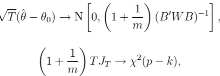
θ JT = [HT(θ0)−HN(θ)]
0W[HT(θ0)−HN(θ)],
whereW−1 is the covariance matrix ofHT(θ0). Denoting the solution
and Singleton (1993) prove the following asymptotic results:
The objective function JT is minimized using the optimization package OPTMUM programmed in GAUSS language. We apply the Broyden-Fletcher-Glodfard-Shanno algorithm. To compute the co-variance matrix we need to obtain B. Computation of B requires two steps: first, obtaining the numerical first derivatives of the
coef-ficients of the VAR representation with respect to the estimates of the structural parameters θ for each of the m simulations; second, averaging the m-numericalfirst derivatives to get B.
4
DATA AND ESTIMATION RESULTS
We consider quarterly U.S. data for the growth rate of output, the inflation rate obtained from the implicit GDP deflator and the Fed funds rate during the post-Volcker period (1983:1-2008:1). In addi-tion, we also considered real-time data on output growth and
in-flation as reported by the Federal Reserve Bank of Philadelphia.11
Figure 1 shows the five time series considered in the paper.
We focus on the post-Volcker period for two main reasons. First, the Taylor rule seems to fit better in this period than in the pre-Volcker era. Second, considering the pre-pre-Volcker era opens the door to many issues studied in the literature, including the presence of macroeconomic switching regimes and the existence of switches in monetary policy (see, for instance, Sims and Zha, 2006). These issues are beyond the scope of this paper.
1 1
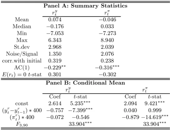
Next, we motivate the inclusion of real-time data in the esti-mated policy rule. As a preliminary step, we analyze whether real-time data are a rational forecast of revised data. Following Aruoba (2008), Panel A of Table 1 shows a set of summary statistics and tests that allow us to assess whether revision processes for output growth and inflation are well-behaved. For both revision processes, we cannot reject the null hypothesis that the unconditional mean is null. However, on the one hand, the standard deviation for the two revision processes is quite large, especially when compared to revised data standard deviations (i.e. noise/signal parameter). On the other hand, the revision processes are likely to show afirst-order autocorrelation pattern. The evidence that revisions are not ratio-nal forecast errors is further supported by the statistics displayed in Panel B. Neither Output growth nor inflation revision processes are orthogonal to the initial announcements and their conditional means are not null.
These preliminary estimation results are in line with the empiri-cal evidence provided by Aruoba (2008) whofinds that data revisions for these variables are not white noise. The non-rational features of revision processes shown above, together with the important diff er-ences in estimated parameters values shown below, when real-time and revised data are jointly used in the structural estimation pro-cedure, suggest strong evidence that a policymaker’s decisions could be determined by the availability of data at the time of policy im-plementation. Next, we estimate the extended version of the NKM model by considering both revised and real-time data.
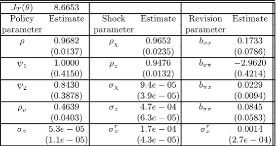
Table 2 shows the estimation results obtained using both revised and real-time data. The inflation parameter estimate is extremely close to one and the output gap coefficient is large and significant. Moreover, the policy inertia parameter estimate (ρ= 0.97) is larger whereas the policy shock persistence parameter though smaller than in previous studies mentioned above is still significant (ρv = 0.46).
evi-Table 1.Revision process analysis. Actual data.
Panel A: Summary Statistics
ryt rtπ
Mean 0.074 −0.046
Median −0.176 0.033
Min −7.053 −7.273
Max 6.343 8.940
St.dev 2.968 2.039
Noise/Signal 1.350 2.076
corr.with initial 0.319 0.238
AC(1) −0.229∗∗ −0.316∗∗∗ E(rt) = 0t-stat 0.301 −0.302
Panel B: Conditional Mean
ryt rtπ
Coef t-stat Coef t-stat const 2.614 5.235∗∗∗ 2.094 9.421∗∗∗
(yrt−yr
t−1)∗400 −0.757 −7.399∗∗∗ 0.040 0.999
(πrt)∗400 −0.072 −0.546 −0.879−14.619∗∗∗
F3,90 33.904∗∗∗ 33.904∗∗∗
dence provided by Aruoba (2008) and that shown in Table 1 (Panel B). In particular, the coefficient of inflation in the output revision equation is large and significant (bxπ =−2.96). Finally, we also ob-serve that the estimated standard deviation of innovations associated with output revision is much higher than the one associated with
in-flation revision process innovations.
Table 2.Joint estimation of the NKM model and the revision processes using both revised and real-time data.
JT(θ) 8.6653
Policy Estimate Shock Estimate Revision Estimate parameter parameter parameter
ρ 0.9682 ρχ 0.9652 bxx 0.1733
(0.0137) (0.0235) (0.0786) ψ1 1.0000 ρz 0.9476 bxπ −2.9620
(0.4150) (0.0132) (0.4214) ψ2 0.8430 σχ 9.4e−05 bπx 0.0229
(0.3878) (3.9e−05) (0.0094) ρv 0.4639 σz 4.7e−04 bππ 0.0845
(0.0403) (6.3e−05) (0.0583) σv 5.3e−05 σrπ 1.7e−04 σrx 0.0014
(1.1e−05) (4.3e−05) (2.7e−04)
Under the null hypothesis, H0 : bxx = bxπ = bπx = bππ = 0,
rx
t and rxt can be viewed as rational forecast errors. That is, this
hypothesis implies that the two revision processes are characterized by two white noise processes r
xtand rπt. Should revisions of real-time
data be rational forecast errors, then the arrival of revised data would not be relevant for policy makers’ decisions and policy rule estimates would be rather similar using either revised or real-time data. In order to analyze whether the characteristics of revision processes have an effect on estimated policy rule parameters, we then estimate the system under the null hypothesis that rx
t and rxt are rational
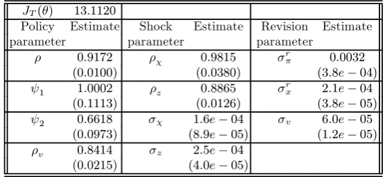
Table 3 shows the estimation results imposing H0. It is well known that the null hypothesisH0 can be tested using the following Wald statistic
F1 =
µ
1 + 1 m
T[JT(θ)−JT(θ0)]→χ2(4),
where JT(θ0) denotes the value of the distance function under H0.
F1-statistic takes the value 432.2. Therefore, we can reject the joint hypothesis that the revision processes of output and inflation are both white noise processes at any standard significance level.
Comparing the estimation results of Tables 2 and 3, it is inter-esting to observe that policy inertia and output gap coefficients (ρ
andψ2) decrease when imposing the restriction that the two revision processes are well-behaved, i.e. when H0 is imposed. Although the reduction in the latter is not statistically significant. Moreover, the policy shock persistence parameter, ρv, increases by imposing H0.
These results obtained under H0 are in line with the estimates of these parameters obtained in previous papers that use only revised data.
Furthermore, it is interesting to note that imposingH0 leads to some poor estimates of the standard deviations of the two revision processes (i.e.σr
x andσrπ). Thus, the estimate of the standard
devia-tion of inflation revision isfifteen times larger than the one associated with output revision. These estimation results are in sharp contrast with those displayed in Table 2, but also with the actual statistics reported by Aruoba (2008, Table 1), which show that actual output revision volatility is twice as large as inflation revision volatility.
model underestimates the standard deviation of the revision process. With such a low standard deviation, for only 40% of the simulated series, we could not reject the hypothesis that the unconditional mean is null. We also find evidence of an autocorrelation pattern, and the conditional mean is different from zero. Using simulated data, all real-time variables seem to play a role in explaining the output growth revision process, which confirms the hypothesis that this revision process is not a rational forecast error. For inflation, we again underestimate the standard deviation of the revision process. The latest result is driven by the low estimate for the standard devia-tion of the innovadevia-tion associated with the inflation revision process. Consistent with actual data, the conditional mean of the inflation revision process is also different from zero using simulated data.
Table 3.Joint estimation of the NKM model assuming that the revision processes are well-behaved.
JT(θ) 13.1120
Policy Estimate Shock Estimate Revision Estimate parameter parameter parameter
ρ 0.9172 ρχ 0.9815 σrπ 0.0032
(0.0100) (0.0380) (3.8e−04) ψ1 1.0002 ρz 0.8865 σrx 2.1e−04
(0.1113) (0.0126) (3.8e−05) ψ2 0.6618 σχ 1.6e−04 σv 6.0e−05
(0.0973) (8.9e−05) (1.2e−05) ρv 0.8414 σz 2.5e−04
(0.0215) (4.0e−05)
Table 4.Output growth revision process analysis. Simulated series.
Panel A: Summary Statistics
percentile
Av.Coef 1 5 10 50 90 95 99
Mean 0.000 −0.061−0.041−0.031 0.001 0.032 0.040 0.050
Median −0.001 −0.245−0.176−0.144−0.004 0.142 0.179 0.227
Min −3.515 −5.323−4.633−4.325−3.428−2.801−2.696 −2.341
Max 3.511 2.410 2.674 2.861 3.440 4.279 4.655 5.094
St.dev 1.403 1.156 1.241 1.276 1.400 1.540 1.572 1.666
Noise/Signal 5.583 4.451 4.793 4.929 5.565 6.250 6.495 6.735
corr.with initial 0.462 0.319 0.362 0.382 0.467 0.531 0.553 0.593
AC(1) −0.248 0.478 0.956 1.362 2.403 3.222 3.396 3.618∗∗∗ E(rt) = 0t-stat 0.003 0.020 0.031 0.190 0.445 0.506 0.641
Panel B: Conditional Mean
percentile t-stats
Av.Coef 1 5 10 50 90 95 99
const 0.562 3.578 4.296 4.745 6.719 9.524 10.487 12.129∗∗∗
(yrt−yrt−1)∗400 −0.895 49.167 56.405 60.062 75.245 93.617 100.849 117.126∗∗∗
(πrt)∗400 −0.219 3.379 4.398 4.842 7.035 9.728 10.852 12.726∗∗∗
F3,90 1163.8 1355.1 1427.1 1873.7 2449.3 2693.5 2967.4∗∗∗
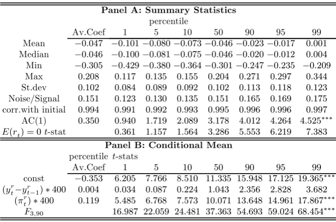
Table 5.Inflation revision process analysis. Simulated series.
Panel A: Summary Statistics
Max 0.208 0.117 0.135 0.155 0.204 0.271 0.297 0.344
St.dev 0.102 0.084 0.089 0.092 0.102 0.113 0.118 0.123
Noise/Signal 0.151 0.123 0.130 0.135 0.151 0.165 0.169 0.175
corr.with initial 0.994 0.991 0.992 0.993 0.995 0.996 0.996 0.997
AC(1) 0.350 0.940 1.719 2.089 3.178 4.012 4.264 4.525∗∗∗
E(rt) = 0t-stat 0.361 1.157 1.564 3.286 5.553 6.219 7.383
Panel B: Conditional Mean
percentile t-stats
Av.Coef 1 5 10 50 90 95 99
const −0.353 6.205 7.766 8.510 11.335 15.948 17.125 19.365∗∗∗
(yrt−y r
t−1)∗400 0.004 0.034 0.087 0.224 1.043 2.356 2.828 3.682
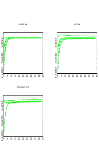
(i.e. using the estimates displayed in Table 3). The size of the shock in each case is determined by its estimated standard deviation. In all cases, we observe that the size of the impulse responses is larger underH0, and is significantly different (i.e. the impulse response lies outside the confidence bands) in the cases of the interest rate im-pulse response to any shock and the imim-pulse-responses of output gap and inflation to a productivity shock. More important, the interest rate impulse response to a restrictive (positive) monetary policy in-novation under H0 is quite unrealistic because it leads to a negative response of the interest rate that is due to the large negative re-sponses of both output gap and inflation that dominate the positive effect induced by the policy innovation.
5
CONCLUSIONS
This paper suggests an augmented version of the New Keynesian Monetary (NKM) model, which contemplates revision processes of output and inflation data in order to (i) test whether initial an-nouncements are a rational forecast of revised data in the context of a structural model and, (ii) assess the influence of deviations of real time data from being a rational forecast of revised data on the estimated monetary policy rule parameters.
The estimation results show that the policy inertia parameter in the policy rule becomes even larger, whereas policy shock persistence substantially decreases by allowing for the possibility that the initial announcements are not a rational forecast of the revised data. More-over, the estimation results indeed show that many revision process parameters are significant, suggesting that real-time data are not rational forecasts. In particular, the coefficient of inflation in the output revision equation is large and significant. Furthermore, the estimation results show that the innovations associated with output revision are much higher than the inflation revision process innova-tions.
References
1. Aruoba, Borogan S. (2008).“Data revisions are not well-behaved”, Journal of Money, Credit and Banking40, 319-340.
2. Clarida, Richard, Jordi Galí, and Mark Gertler (2000) “Monetary policy rules and macroeconomic stability: evidence and some theory,” Quarterly Journal of Economics 115, 147-180.
3. Croushore, Dean, and Tom Stark (2001) “A real time data set for macroecono-mists”,Journal of Econometrics105,111-130.
4. Diebold, Francis X., Glenn D. Rudebusch (1991) “Forecasting output with the composite leading index: an ex ante analysis,”Journal of the American Statistical Association86, 603-610.
5. Duffie, D., and K. J. Singleton (1993), “Simulated moments estimation of Markov models of asset prices,”Econometrica61, 929-952.
6. English, William B., William R. Nelson, and Brian P. Sack (2003)."Interpreting the significance of the lagged interest rate in estimated monetary policy rules",The B.E. Journal in Macroeconomics, Contributions to Macroeconomics 3(1), Article 5.
7. Gerlach-Kristen, Petra (2003) “Interest rate smoothing: monetary policy or unob-served variables?”The B.E. Journal in Macroeconomics, Contributions to Macro-economics4(1), Article 3.
8. Ghyssels, Eric, Norman R. Swanson, and Myles Callan (2002) “Monetary policy rules and data uncertainty,”Southern Economic Journal 69, 239-265.
9. Gouriéroux, C., E. Renault, and N. Touzi (2000), “Calibration by simulation for small sample bias correction,” in Mariano, R., T. Schuermann and M. Weeks (eds.) Simulation-Based Inference in Econometrics, Methods and Applications. Cambridge University Press, Cambridge.
10. Kavajecz, Kenneth A., and Sean S. Collins (1995) “Rationality of preliminary money stock estimates,”Review of Economics and Statistics 77, 32-41.
11. Lee, B. S., and B. F. Ingram (1991), “Simulation estimation of time-series models,” Journal of Econometrics47, 197-205.
12. Lubik, Thomas A., and Frank Schorfheide (2003) “Computing sunspot equilibria in linear rational expectations models,”Journal of Economics Dynamics and Control 28, 273-285.
13. Mankiw, N.Gregory, David E. Runkle, and Matthew D. Shapiro (1984) “Are pre-liminary announcements of the money stock rational forecasts?”Journal of Mon-etary Economics14, 15-27.
14. Maravall., Agustín, and David A. Pierce (1986) “The transmission of data noise into policy noise in US monetary control,”Econometrica 54, 961-979.
15. María-Dolores, Ramón, and Jesús Vázquez (2006) “How the New Keynesian mon-etary modelfits in the US and the Euro area? An indirect inference approach,” The B.E Journal in Macroeconomics, Topics in Macroeconomics 6 (2) Article 9. 16. María-Dolores, Ramón, and Jesús Vázquez (2008) “Term structure and estimated
monetary policy rule in the Eurozone,”Spanish Economic Review 10, 251-77. 17. Orphanides, Athanasios (2001) “Monetary policy rules based on real-time data,”
American Economic Review 91, 964-985.
18. Rudebusch, Glenn D. (2002) “Term structure evidence on interest rate smoothing and monetary policy inertia,”Journal of Monetary Economics 49, 1161-1187. 19. Sims, Christopher A., Tao Zha (2006) “Were there regime switches in U.S.
20. Smith, Anthony A. (1993) “Estimating nonlinear time-series models using simu-lated vector autoregressions,”Journal of Applied Econometrics 8, s63-s84. 21. Smith, Anthony A. (2008) “Indirect inference,”The New Palgrave Dictionary of
Economics, 2nd Edition (forthcoming).
22. Trivellato, U. and E. Rettore. (1986) “Preliminary data errors and their impact on the forecast error of simultaneous equation models,”Journal of Business and Economic and Statistics4, 445-453.