Conservative formulation of unsteady pipe-flow model for water in its liquid form.

(1)

(2)

This content has been downloaded from IOPscience. Please scroll down to see the full text.

Download details:

IP Address: 202.94.83.93

This content was downloaded on 06/06/2017 at 09:45

Please note that terms and conditions apply.

View the table of contents for this issue, or go to the journal homepage for more

(3)

1

Content from this work may be used under the terms of theCreative Commons Attribution 3.0 licence. Any further distribution of this work must maintain attribution to the author(s) and the title of the work, journal citation and DOI.

Published under licence by IOP Publishing Ltd

1234567890

Conference on Theoretical Physics and Nonlinear Phenomena 2016 IOP Publishing IOP Conf. Series: Journal of Physics: Conf. Series 856_{(2017) 012014} _{doi :10.1088/1742-6596/856/1/012014}

Conservative formulation of unsteady pipe-flow

model for water in its liquid form

Bambang Supriyadi1

, I Gusti Ketut Puja2

, F A Rusdi Sambada2

and Sudi Mungkasi3

1_{Department of Civil and Environmental Engineering, Faculty of Engineering, Gadjah Mada}

University, Jalan Grafika No. 2, Yogyakarta 55281, Indonesia

2_{Department of Mechanical Engineering, Faculty of Science and Technology, Sanata Dharma}

University, Mrican, Tromol Pos 29, Yogyakarta 55002, Indonesia

3_{Department of Mathematics, Faculty of Science and Technology, Sanata Dharma University,}

Mrican, Tromol Pos 29, Yogyakarta 55002, Indonesia

E-mail: bbsupri@tsipil.ugm.ac.id, ketut@usd.ac.id, sambada@usd.ac.id, sudi@usd.ac.id

Abstract. We consider flows in a pipe system. The problem relating to the pipe system usually occurs in real life as well as in the laboratory, such as in the distillation process. This unsteady problem can be modeled into a hyperbolic system of partial differential equations. Our goal is to propose the use of a conservative finite-volume numerical method for solving the unsteady pipe-flow model. We obtain that the method is able to solve the pipe-flow problem successfully.

1. Introduction

Pipe flows occur in daily life as well as in the laboratory. In the laboratory, pipe flows can be found in the water distillation process. Distillation itself includes two types of water forms, gas and liquid.

Mathematical models for pipe flows have been available in the literature [1]. In the gaseous form, Mungkasi [2] used a conservative finite-volume numerical method for solving the Euler equations of gas dynamics. In the liquid form, ˇSkifi´c et al [3] proposed a nonconservative formulation of unsteady pipe-flow problems. The conservative formulation for water in its liquid form was not given in the work of ˇSkifi´cet al [3].

This paper complements the work of ˇSkifi´c et al [3]. We propose the use of a conservative formulation of unsteady pipe-flow model for water in its liquid form. Because the model is hyperbolic, we choose a finite-volume method as our conservative formulation to solve the model. Finite-volume methods have been well known as powerful methods to reconstruct smooth and nonsmooth functions as solutions to problems [4].

(4)

2 2. Mathematical model

In this section, we write the mathematical model and the general formulation for solving the model. We assume that the model is one-dimensional.

The mathematical model governing conservation laws of water flowing in a pipe [3] is

Ht+

c2

gAQx= 0, (1)

Qt+gAHx = 0. (2)

Here, the involved variables and parameters are as follows: tis the time variable,x is the space variable for coordinate along the conduit length, H = H(x, t) denotes the piezometric head,

Q=Q(x, t) represents the discharge,Ameans the pipe cross-sectional area,cis the wave speed, and g is the acceleration due to gravity. In this paper, we assume that there is no head losses in the system.

Equations (1) and (2) can be written in the vector form of conservation laws

ut+f(u)_x=0, (3)

where the vector of conserved quantities is

u=

and the vector of flux functions is

f(u)=

The Jacobian matrix of the vector of flux functions is defined as

A(u)= ∂f

with eigenvalues and right eigenvalue vectors are

λ(1),(2)=∓c (7)

Now, suppose that we have the scalar conservation law of (3), that is

ut+f(u)x = 0, (9)

where u is a scalar (not a vector). The corresponding fully discrete finite-volume numerical scheme is

Qn_i+1 =Qn_i − ∆t

∆x(F

n

i+1/2−Fi−n1/2), (10) where ∆x is the cell width, and ∆tis the time step in a finite-volume framework. Here, Un

i is the finite-volume average approximation of the quantity at theith cell at thenth time step, and

Fn

(5)

3 1234567890

3. Numerical method

As follows, we briefly describe the numerical method that we use to solve (1) and (2). The method is a finite-volume method, which is conservative.

Let us consider (3). Using the standard finite-volume framework, let ∆x be the cell width of uniformly discretized space domain, and ∆tbe a given time step. In the semidiscrete form, the finite-volume method is

d

dtUj(t) =−

1

∆x(Fj+12(t)−Fj−12(t)) (11)

where U is the vector of approximate conserved quantities and Fis the vector of approximate fluxes. This scheme is called semidiscrete because we have discretized the equations with respect to space, but the time variable is still continuous.

To evolve the conserved quantity, we need to integrate the semidiscrete form (11) with respect to time. We can use any standard method for solving ordinary differential equations (ODEs). As we have used a first-order method in space, we choose to use a first-order method in time. Note that a higher order method in time is not needed because we have used a first-order method in space. In this paper, we implement the first-order Runge-Kutta method (the Euler method) to integrate the semidiscrete form (11) with respect to time. The fully discrete finite-volume method is

The flux is approximated using the Lax–Friedrichs formulation (see LeVeque [5] for more details):

Here we have dropped the superscript n for brevity of writing. Considering the Courant-Friedrichs-Lewy (CFL) condition, we do the numerical computation in such a way that the numerical method is stable.

4. Numerical results

In this section we present some numerical results to show that the numerical method works well for solving (1) and (2). All measured quantities are assumed to be in SI units with the MKS system.

The boundary conditions at x= 0 are

H(0, t) = 10, Q(0, t) = 1, (16)

and at x= 1200 are

(6)

4

0 200 400 600 800 1000 1200

10 15 20 25 30 35 40 45

x−position

H(x,t)

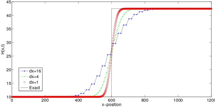
dx=16 dx=4 dx=1 Exact

Figure 1. Results for varying cell width ∆x at time t = 0.4 with dx meaning ∆x. Here ∆t= ∆x/2c. The numerical solutions converge to the exact solution as ∆x approaches zero.

With these settings, we simulate the problem to obtain numerical solutions at time t= 0.4 and analyze the results.

Based on simulation results, the presented numerical method is diffusive. However, the diffusion can be reduced by taking more computational cells, that is, taking a smaller cell width ∆x, as shown in figure 1. (To generate this figure, we take ∆t= ∆x/2cfor our numerical simulations.) This could make the computation more expensive, but in fact it is not too expensive due to the nature of the first-order numerical method and the model. We observe that taking smaller ∆xleads to more accurate numerical solution. Therefore, by numerical experiments our numerical method converges to the exact solution, as the cell width tends to zero. We observe that taking the time step ∆t >∆x/cresults in an unstable method.

5. Conclusion

We have proposed the use of the conservative finite-volume method to solve the water flow problem in a pipe. The method is simple in structure, because it is explicit. The method is conditionally stable. Our results are limited to one-dimensional problems. Possible future direction may extend these results for multidimensional problems.

Acknowledgments

This research was financially supported by Sanata Dharma University and a research grant from

Direktorat Riset dan Pengabdian Masyarakat(DRPM) of Ministry of Research, Technology and Higher Education of the Republic of Indonesia year 2016.

References

[1] Chaudhry M H 1987Applied Hydraulic Transients(New York: Van Nostrand Reinhold) [2] Mungkasi S 2016AIP Conf. Proc.1737₀₄₀₀₀₂

(7)

5 1234567890

[4] Mungkasi S 2016Adv. Math. Phys.20167528625