APPLICATION OF GIS AND GROUNDWATER MODELLING TECHNIQUES TO
IDENTIFY THE PERCHED AQUIFERS
TO DEMARKATE WATER LOGGING CONDITIONS IN PARTS OF MEHSANA
D . Rawala, A.Vyas a, S.S.Rao a.
a CEPT University, Ahmedabad, India - [email protected],[email protected], [email protected]
Commission VIII, WG VIII/4
KEY WORDS: Ground Water, Hydrological Cycle, Geology, Rainfall. Piezometer.
ABSTRACT:
Groundwater is very important component of the hydrological cycle. It is an important source of water for drinking, domestic, industrial and agricultural uses. It plays a key role in meeting the water needs of various users sectors in India. Ground water resource is contributed by two major sources – rainfall and the other seepage from irrigation of the crops. A man-made effort through artificial recharge for water conservation structures adds to the ground water. The ground water behaviour in Indian sub-continent is highly complicated due to the occurrence of diversified geological formations with considerable lithological and chronological variations, complex tectonic framework, climatological dissimilarities and various hydro-chemical conditions. Assessment of ground water resources of an area requires proper identification and mapping of geological structures, geomorphic features along with sound information regarding slope, drainage, lithology, soil as well as thickness of the weathered zones.
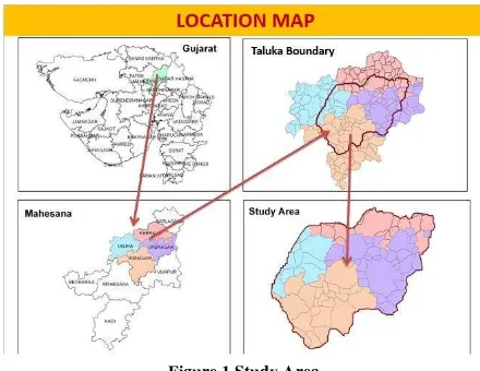
This study is to understand the ground water scenario in the water logged areas of Dharoi command while the surrounding areas showing continuous decline of water levels. The area falls in the command area of Dhorai dam and is in Mehsana District of Gujarat State. A part of northern command of Dharoi Command area falls in hard rock areas while the lower and southern portion fall in alluvial areas in the Dharoi Command (RBC) area in Mahsana Mehsana District of the Gujarat State.
The study highlights the application of GIS in establishing the basic parameters of soil, land use and the distribution of water logging over a period of time and the groundwater modelling identifies the groundwater regime of the area and estimates the total recharge to the area due to surface water irrigation and rainfall and suggests suitable method to control water logging in the area.
1. INTRODUCTION
Assessment of ground water resources of an area requires proper identification and mapping of geological structures, geomorphic features along with sound information regarding slope, drainage, lithology, soil as well as thickness of the weathered zones. Amongst the latest available technologies, the remote sensing technique along with Geographic Information System (GIS) has acquired the supreme position over the conventional methods in studying the hydrogeology due to its synoptic view, repetitive coverage, and high ratio of benefit to cost and availability of data in different wavelength ranges of the electromagnetic spectrum. Through digital image processing of the remotely sensed satellite images, the controlling features of ground water can be identified accurately and thus the terrain can be classified properly in terms of ground water potentiality and prosperity. Geographic Information System (GIS) has been found to be one of the most powerful techniques in assessing the suitability of land based on the spatial variability of hydro geological parameters. GIS offers many tools to extract the information about the ground water prospect of an area by integrating information regarding geologic structures, geomorphology, soil, lithology, drainage, land use, vegetation etc.
Gujarat is the seventh largest state of India, situating in the Western part of the country is largely an arid state for most of its part. In the mountainous hard rock terrain of Aravalli, ground water is the only source of water in the northern part of the Gujarat. A part of Northern command of Dharoi command area falls in hard rock areas while the lower and southern portion fall in alluvial areas. Due to the combination of hard rock areas and the perched water table conditions occurring
due to the occurrence of clay at very shallow depths in parts of the Dharoi Command (RBC) in Mahesana District of the Gujarat state particularly in Kheralu, Vadnagar, Visnagar and Unjha Talukas have water logging conditions. The objective of this study is to understand the hydrogeology of the terrain and its influence in ground water and then to develop an appropriate ground water modelling using Visual Modflow to delineate the water logging areas and suggest suitable methods to recharge the lower aquifer and estimate the approximate amount of water that can be recharged in the area.
2. OBJECTIVE
To delineate the aerial extent of the perched aquifer and study the geohydrological characteristics of perched and deeper aquifer system.
To quantify the ground water withdrawal and recharge input potential of layered aquifer system and assess its
adverse effects due to shallow water levels.
To develop a mathematical model of Part of Vadnagar, Visnagar and Kheralu and Unjhataluka of Mahesana district of North Gujarat Region representing perched aquifer system (approximately 605 Sq.Kms).
3. STUDY AREA
and Unjha Talukas. The location of the study area is shown in the map below:
3.1 Physiography and Drainage
The study area has a diverse landscape. It is characterized by hilly upland in the northeast, followed by piedmont zone with shallow alluvium and residual hills/inselbergs, and rolling to gently sloping vast Alluvial-Eolian plain. The elevation in the study ranges from less than 95 meters in the southwestern part, and 194 meters above mean sea level (AMSL) in the north-eastern part. The master slope is towards southwest. The higher elevations in the study are attained by hills in the northwest.
3.2 Climate:
The district has semi-arid climate. Extreme temperatures, erratic rainfall and high evaporation are the characteristic features of this type of climate. The climate of the district, like other parts of North Gujarat, is dominated by hot summer, cold winter, meagre rainfall and a general dryness except during the short monsoon period. The year may be divided into four seasons. The period from March to mid-June is the hot summer season followed by south-west monsoon which lasts till September. October and November are the post-monsoon months when the temperatures rise again. The winter season starts from December and ends in February.
3.2.1 Rainfall:
The average rainfall in the area is about 660.42 mm. The standard deviation is about 331.57 indicating that the coefficient of variation is almost 50 %. It shows that the rainfall is highly irregular and cannot be depended upon. It is mainly concentrated during June to September months. The annual variation of rainfall is shown below
3.2.2 Temperature: After mid-March there is a rapid rise in temperature and May is the hottest month with mean daily maximum temperature of 41.70C and mean daily minimum
temperature of 25.30C. In hot season strong dust laden scorching winds blow on many days and the weather becomes uncomfortable. On individual days, the day temperature may go above 450C.
After October, both night and day temperatures decrease. January is the coldest month with mean daily maximum and minimum temperature of 28.40C and 10.70C respectively. During the winter season the district is affected by cold waves associated with western disturbances. On such occasions the minimum temperature may drop down to 1 or 2 degrees below freezing point. The highest and lowest temperatures recorded at Deesa are 500C (15th May 1912) and 2.20C (15th Jan 1935).
3.2.3 Humidity: During the monsoon period the humidity is between 60-80%. On an average, humidity is low during the year. The driest period of the year occur during winter and summer seasons when relative humidity in the afternoon is less than 30%.
3.2.4 Surface Water Resources: The study area is deficient in respect of surface water resources. There are no perennial rivers flowing through the study area and thus the water resources are dependent mainly on the surface run-off and river flows during monsoon period. In order to harness surface water resources, major and medium irrigation projects were planned and executed. The existing irrigation schemes and command area of Dharoi command canal in the study are shown in the map.
Figure 1 Study Area
Figure 3 Elevation and Natural Drainages
3.2.5 Land Utilization Pattern: The total area reported for
Above table represents the category-wise land use derived
from the respective years’ satellite imagery. The study area is
656.28 sq.km. Comparisons made between Land Use which is carried out from the Satellite images of year 1998 and 2008. Area under agriculture is decreasing, the built up area also increase. Agriculture in this region depends mainly on rainfall. The fallow land has marginally decreased. Differences are seen in the above table that Waste lands are increasing because of water logging. With increase in the Salinity, land is under cultivation and more than 65% of its working population engaged in agriculture and agro related activities. Months of sowing and harvesting of major crops in this region Wheat is the major crop grows between the months of October and March. The second important crop is Jowar, which is grown between August and December months. The cash crops, groundnut and cotton are also grown in the study region.
3.3 Hydrogeology:
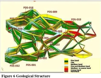
3.3.1 Geology and sub-surface Geology: The total area falls in quaternary alluvial deposits of more than 400 m depth with more than 4 major aquifer formations. The aquifers are mainly alluvial formations except in the North East portion of the area where basement rock is exposed at about 35- 50 to m depth. The geology of Dharoi canal command area is shown below. It shows that the aquifers in the North are hard rock, valley fills in the middle and the older alluvium in the extreme south.
Generally the groundwater moves and follows the topography in unconfined aquifers those move from North East to South West in the study area.. In northeast and in west part basement is observed at shallow depth. The clay layers are thick and dominant in the area. Sand layers are thin in lenses form. The panel diagram obtained from the litho logs of the tube well of percentage of clay available in the area.
3.4 Ground Water in Fissured Formations (Hard Rocks) : Primarily the thickness and extent of weathering zones, and size and interconnection of fissures and joints, which provide secondary porosity, govern occurrence and movement of ground water in the hard rocks. The high hills, in general, act as run off zone because of steep gradients and impervious nature of formations. Only in low lying terrain and intermountain valleys, ground water occurs in shallow weathered and fractured zones under water table to semi-confined conditions. In such areas the blown sand occurs as thin capping.
These formations, in general, do not form good repository of ground water. The depth of wells ranges from 8 to 18.5 m below ground water level and depth to water level in open wells varies from 5 to 14 m below ground water level. The water table is shallow near streams and topographically low areas. Yield of wells ranges from 30 to 120 m³/day with an average of 75 m3/day. Open wells generally sustain intermittent pumping during summer season.
3.4.1 Ground Water In alluvial formations:
of formations. Only in low lying terrain and intermountain valleys, ground water occurs in shallow weathered and fractured zones under water table to semi-confined conditions. In such areas the blown sand occurs as thin capping.
These formations, in general, do not form good repository of ground water. The depth of wells ranges from 8 to 18.5 m below ground water level and depth to water level in open wells varies from 5 to 14 m below ground water level. The water table is shallow near streams and topographically low areas. Yield of wells ranges from 30 to 120 m³/day with an average of 75 m3/day. Open wells generally sustain intermittent pumping during summer season.
3.4.2 Ground Water In alluvial formations:
Major part of the study area is underlain by post-Miocene alluvium and older sedimentary formations. These sediments mainly consist of fine to coarse-grained sand, gravel, silt, clay, clay stones, siltstones and grit. Thickness of alluvium gradually increases from piedmont zone in the northeast towards west and southwest. Maximum thickness of alluvium in the district is estimated to be about 550-600 m in the central part.
Ground water occurs both under phreatic and confined conditions within sedimentary formations. The occurrence and movement of ground water is mainly controlled by inter-granular pore spaces. Two major aquifer units identified.
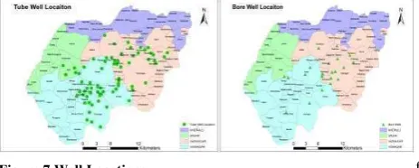
Ground water is extensively developed by dug, dug-cum-bored and tube wells in areas underlain by alluvium. Depth of dug and dug-cum-bore wells ranges from 5 m to 65 m below ground water level whereas depth to water level, in general, varies from 10 to 20 m below ground water level. Deeper water table, between 20 and 32 m below ground water level, however, is observed in the central part, south of Saraswati River, and in the eastern part. In such areas, the dug section of the wells is generally dry and ground water is extracted directly from the bores and/or tube wells that generally tap deeper aquifers. Depth to water level in phreatic aquifer is shallow, less than 10 m, in command areas of Dharoi covering parts of Patan and Kheralu, Visnagar, Mahesanatalukas. Also in entire southwestern part, where ground water is saline, water levels are shallow. In such areas dug wells are rare and/or located in or vicinity of ponds. Ground water development using dug wells and/or shallow bore wells in phreatic aquifer is limited because of salinity in major part, deep water levels and limited saturated water column and/or major yields in some areas also to some extent presence of high yielding deep aquifers. Such areas are confined and localized in parts of Kheralu. The yield of wells is generally low to moderate and ranges from 200 to 800 m3/day for 3 to 5 m drawdown.
The tube wells are the main groundwater withdrawal structures in the district and range in depth from 60 m to 350 m. Shallow tube wells (<100 m) are restricted to the alluvial area in the northeast, mainly in parts of Kheralu and Vijapurtalukas. In the central, southwestern and southern parts, deep tube wells tap one or more aquifers. The depth to piezometric surface of deep confined aquifers ranges from near surface in the southwestern part to more than 120 m bgl in the central part. The discharges of tube wells vary from 20 to 60 lps for 8m to 13 m of drawdown. The average yield of a 250 m deep tube well is around 20 lps. The transmissivity of deeper aquifer varies from 300 to more than 1200 m2/day.
A very rapid pace of ground water development from deep aquifers over the years with practically no control in the use pattern combined with prolonged years of deficit rainfall particularly in eighties has resulted in tremendous lowering of the piezometric surface. This has resulted in well failures, lowering of discharge and increased depth of tube wells over the years.
Ground water levels and ground water quality in Aquifer A1 of water logged area of Dharoi RBC, 22 numbers of open wells are fixed in year 2009.The locations of the wells are presented in above figure these structures are monitored monthly for water level measurement and water sampling.
3.4.3 Behaviour of Water Levels in Unconfined Aquifer-A1: The thematic map showing the land use patterns, drainage, soils etc are prepared in GIS environment, the thematic layers on dynamic data in terms of water level and quality variation over the space and time, the information collected is validated as base level information and using this layer important assessment on changes due to recharge activities envisaged under study. The spatial and temporal analysis has been considered for the dynamic data..
Figure 8 Average Water Level
The total dissolved solids in the prevailing groundwater vary from less than 1000 ppm to more than 4500 ppm in the water logged areas depending on the level of water logging. The maximum concentration 4500 ppm is found in the southern western part of the study area during the monsoon, Rabi seasons and in a summer it is concentration in only center part of the study area and villages of Visnagar and Vadnagar Talukas. Groundwater quality maps for different seasons have been prepared to study the variation in seasons and years.
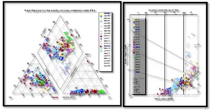
The quality of water has been analyzed using Wilcox classification to study the usability water for irrigation.The data of PDS wells in the study area are plotted using Aquachem software. The results indicate that 2/3rd of samples fall in c3-c4 and s2 to s3 zones indicating the groundwater is highly prone to salinity and sodium hazard. This appears mainly to water logging in the area and not suitable for irrigation.
3.5 Groundwater Modelling : Modelling is an attempt to replicate the behaviour of natural groundwater or hydrologic system by defining the essential features of the system in some controlled physical or mathematical manner. Modelling plays an extremely important role in the management of hydrologic and groundwater system.
The reliability of any groundwater model depends on a proper simulation of the groundwater situation in the basin. This depends on proper calibration, for which the availability of the data on the geometry and hydraulic characteristics of the aquifer and data on water levels and the water balance are indispensable.
3.5.1 The Conceptual Model: References from Other Literature:
The study area has been demarked based on the canal distribution, water logged area and drainage pattern of the area.
It is observed that even though, the area is having more than 20 aquifer zones and has a depth of more than 300 to 400 m, as the problem is of water logging, it is proposed to study the shallow aquifers in detail, to estimate the scope of artificial recharge to deeper aquifers, in the beginning and subsequently moredepths if required. The aquifer sequence proposed study is shown.
The surface contours are drawn based on DEM
The initial water levels are collected from the dug wells /DCBs.
The unconfined groundwater flows mainly from NE to SW of the area.
The North boundary in general is constant boundary A part of North East is considered as General Head
boundary as they are in likelihood of recharge from Northern side.
A part of South West is Constant head boundary
The remaining area outside the study area is considered as no flow boundary.
The inside of the study area is considered as Active area.
3.5.2 Ground-Water Flow Equation: The partial-differential equation of ground-water flow is given as under:
( McDonald and Harbaugh,1988).
Where,
Kxx , Kyy , and Kzz are values of hydraulic conductivity along the x, y, and z coordinate axes, which are assumed to be parallel to the major axes of hydraulic conductivity (L/T); h is the potentiometric head (L);
W is a volumetric flux per unit volume representing sources and/or sinks of water, with W<0.0 for flow out of the ground-water system, and W>0.0 for flow in (T-1);SS is the specific storage of the porous material (L-1); and t is time (T).Even though, the groundwater equations have been developed considering homogeneous aquifers, in general, they do not occur in real life situations. The conductivity values vary considerably in all the directions as well as the Storability values also vary considerably. In normal modelling designs, kx and ky values are taken as same unless otherwise specifically obtained and observed in pumping test data and the vertical permeability data is considered about 10 times less than the horizontal permeability and calibrated subsequently to check these values.
The basic idea of the finite difference method is that the model area is subdivided into a number of sub-areas or polygons. Two families of straight parallel lines make the simplest type of polygon networks, to the x and y direction, respectively, which together form a mesh of rectangles as shown below.
The value of the H at nodal point (i,j) of the mesh is the average of values of nodal points of (i-1,j; I,j-1; i+1, j; I,J+1). This value is obtained by no of iterations as specified by the model builder or as per the requirement of the model.
3.5.3 Grid design: The entire study area has been divided into uniform grid, a number of layers with uniform thickness created. At the time of translating conceptual model to the numerical model, the properties will be assigned to the appropriate grid cells to represent hydrological structure. Grid cells above the topmost hydrological layer (and below the bottommost layer) are set as inactive. This grid is useful for transport where it is desirable to have fine vertical discretization. For this study we have 78 columns (39 kms) and 66 rows (33 kms) with an average grid size of 500 m. The Model Study area is shown below.
3.5.4 The base and top of the aquifer:
However, as the study is restricted to the top few layers to study the effect of water logging and also to see whether the recharge from upper unconfined aquifer to lower confined aquifers, the total thickness has been clubbed to only 6 layers. The first 5 layers are kept as per the actual occurrence and the remaining all the layers are clubbed as one aquifer (6th layer). 3.5.1 Boundary conditions:
The boundary conditions are very important to identify the groundwater movement, the availability of water resources and any predictions thereof.
Broadly there are as under:
1. Constant head boundary conditions 2. General Head boundary conditions 3. Recharge/ River / Drain boundaries / Wall 4. No flow boundaries
5. Active elements
3.5.2 Model Input data: The model has been designed for steady state and unsteady state groundwater flow. The following inputs for elevations for different aquifers were used in the development of model. The aquifer parameter has been estimated based on the pumping tests conducted on the wells. Different type of the data like elevation of the Aquifer, Water Level and pumping data is included in the model.
The Model has been setup in Non Steady State condition for 365 days running period with monthly recharge values starting from July 1 and different pumping rates during Kharif, Rabi and Summer.
3.5.1 Behaviour of water table contours: The actual initial water table contours and estimated from the model are compared in the beginning of the year to see whether the model is working correctly. If they match reasonably, it can be safely assumed that the results would be acceptable. It is seen that the estimated and actual initial water levels are compared very well.
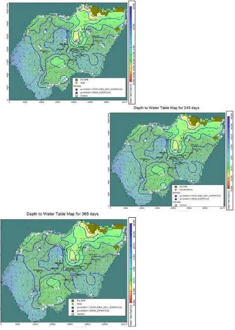
3.6 Surface contours vs. Water: Water logging occurs where ever the surface contours and water table contours intersect. The depth to water table map shows that there are going to be water logging conditions in the South west and central part of the area.
The water table contour map along with surface contours is shown below to see whether any water logging occurs and subsequently to delineate the same. The water table contour map along with surface contours is shown below.
Figure 11 Boundary Condition
Figure 12 Input in the Model
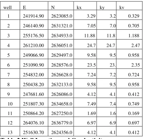
Table 2 Well Location and Conductivity
The equipotential lines for different aquifers for 365 days are given below. For the first unconfined aquifer, the equipotential lines as well as water table contours are drawn to see whether there is any difference between equipotential lines and water table conditions. Broadly they match except in the South Western part of the area.
In the confined conditions, the equipotential lines are similar as no separate initial water levels for different aquifers have been used.
4. RESULTS OF THE MODEL:
The user designates the sub-regions by specifying zone numbers. A separate budget is computed for each zone. The budget for a zone includes a component of flow between each adjacent zone. The zone budget for the whole year (365 days) indicates 1773300 m^3/day of water is coming into the area mainly from storage, constant head, recharge while the same amount is going out of the system from Storage, constant head, wells and through drains. The input and output should normally be equal when the water balance is studies. The contribution of different Zones (aquifers) to the unconfined aquifer is as under:
Table 3 Zone wise and Time wise calcualtion of
Water loggin
Inflow m^3/day Outflow m^3/day Net Balance m^3/day 123 days
Zone 2 to 1 983560 Zone 1 to 2 961830 21730
Zone 3 to 1 511150 Zone 1 to 3 374060 137090 Zone 4 to 1 0 Zone 1 to 4 174.17
246days
Zone 2 to 1 874530 Zone 1 to 2 859780 14750
Zone 3 to 1 429330 Zone 1 to 3 359450 69880 Zone 4 to 1 0 Zone 1 to 4 119.32 -119.32
365days
Zone 2 to 1 766610 Zone 1 to 2 748630 17980
Zone 3 to 1 385030 Zone 1 to 3 359450 25580 Zone 4 to 1 0 Zone 1 to 4 114.8 -114.8
Zone 1= Unconfined aquifer, Zone2 = First confined aquifer
Zone3= Second confined aquifer, Zone 4= Third confined aquifer
The water logged area is considered for different water levels 0 to 10 m, 0 to 7 m and 0 to 5 m mainly during Kharif (123 days). Accordingly the dewatering efforts can be made .The water logged area from 0 to10 m during Kharif season (123 days) is given below.
The water logged area from 0 to 5 m during Kharif season (123 days) is given above. The area of the water logged area is about 127 sq.km.
well E N kx ky kv
1 241914.90 2623085.0 3.29 3.2 0.329
2 246140.90 2631321.0 7.05 7.0 0.705
3 255176.50 2634933.0 11.88 11.8 1.188
4 261210.00 2636051.0 24.7 24.7 2.47
5 249066.90 2629497.0 9.58 9.5 0.958
6 251090.90 2628576.0 23.5 23. 2.35
7 254832.00 2626628.0 7.24 7.2 0.724
8 250438.20 2632133.0 9.58 9.5 0.958
9 247681.60 2626086.0 4.12 4.1 0.412
10 251807.30 2634658.0 7.49 7.4 0.749
11 250864.20 2627250.0 1.69 1.6 0.169
12 264076.10 2636779.0 6.97 6.9 0.697
13 251630.70 2624356.0 4.12 4.1 0.412
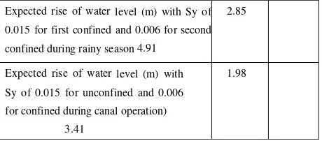
The recharge capabilities in the area has been estimated based on the head difference and the aquifer parameters. The same is shown below for 5 m dewatering in the area both for first confined and second confined aquifers. This has been calculated using the Conductivity values estimated from the pumping test data and the radius of influence of about 500 m for first confined and 1000 m for the second confined aquifers. The rise of water level due to the recharge has been estimated considering the specific yield values of 0.015 for first confined and 0.006 for the second confined aquifers.
Table 4 Calculations
Average thickness of 1st confining clay- m 8 40
Average thickness of IInd aquifer (m)-cinfined first aquifer
13 53
Average thickness of 2nd confining clay 6.5 59.5
Average thickness of 3rd aquifer (m)- 2nd Cinfined aquifer
15 74.5
Average water level in monsoon(m-bgl) 0.5 0.5
Expected Recharge due to construction of Recharge wells in the
Permeability(k)= m/day 8.14 9.9
Radius of well(rw)-m 0.1 0.1
Radius of Influence(r0)-m 250 600
ho( head above the bottom of the aquifer when no pumping is taking - average (m)
48 69
hw (head above the bottom of the aquifer while recharging - average (m)
50.25 71.5
Thickness(b)-m 13 15
Discharge of well(q)-m3/day 191.4 268.5
Discharge of well (q)- lps 2.22 3.11
Radius of influence of each well(r0- (m) 250 600
Area of each well (sq.m) 3.14*r^2 196250 1130400
no of wells per sq.km 5.10 0.88
Reacharge per sq.km per day (cum) 1023.85 Reacharge per sq.km in monsoon (72
days)-cum
73717.36 17100.40
Recharge due to canal of 99 days of Rabi (50 %)
51192.61 11875.28
Total Recharge per year per sq.km-cum 124909.97 28975.69
Total Recharge per year per sq.km-mcm 0.125 0.029
Total Recharge area upto 5 m below Ground level ( sq.km)
127 127
Total expected recharge (mcm) 15.86 3.68
Total No of Recharge wells that can be
constructed in the 127 sq.km area 647 112
Expected rise of water level (m) with Sy of 0.015 for first confined and 0.006 for second
confined during rainy season 4.91 3.68 mcm for the second confined aquifer can be recharged in a year. This will result in about 4.91 rise in first confined aquifer and about 2.85 m rise in the second confined aquifer due to monsoon and about 3.41 m in first confined aquifer and about 1.98 m in the second confined aquifer due to canal recharge.
ACKNOWLEDGEMENTS
Authors like to thank Ground Water Resource Development Corporation LTD, Government of Gujarat for the financial assistance to carry out this project. This paper is an outcome of the study results.
REFERENCES
Sharma and Gupta (1987) have studied the flow of groundwater through different aquifers in Mehsana by tritium study.
Bradley and Phadtare (1989) has studied the aquifers of Mehsana in detail.
Rushton and Tiwari, (1989) have studied the Regional studies of the Mehsana alluvial aquifer regarding the vertical flows and arrived at the conclusion that the vertical flow through clay zones are the ultimate source of most of the water that is pumped from the tube wells and that the horizontal flows account for about 5 % of the abstraction.
Rushton (1990)has reviewed the Methods of estimating the quantity of water leaving the soil zone towards the deeper aquifer in the Mehsana aquifer.
M.V.Patel (1992) has developed a mathematical model for determination of aquifer parameters in alluvial areas with special reference to Rupen Basin, Mehsana.
Columbia Water Centre 2011has conducted surveys to confirm that the groundwater crisis in North Gujarat is severe and likely to get worse.
Majumdar, P. K., Sekhar, M., Sridharan K., Mishra, G. C.(2008)has conducted Numerical simulation of groundwater flow with gradually increasing heterogeneity due to clogging.
N. B. KAVALANEKARA , S. C. SHARMA and K. R. RUSHTON, Dec 2009 have studied the over exploitation of groundwater resources in Mehsana.
P.K.Majumdar(2008) has also modelled the water logging conditions of parts of Rupen basin.