INVESTIGATING THE POTENTIAL OF DEEP NEURAL NETWORKS FOR
LARGE-SCALE CLASSIFICATION OF VERY HIGH RESOLUTION SATELLITE
IMAGES
Tristan Postadjiana, Arnaud Le Brisa, Hichem Sahbib, Cl´ement Malleta
a
Univ. Paris Est, LASTIG MATIS, IGN, ENSG, F-94160 Saint-Mande, France b
CNRS, LIP6 UPMC Sorbonne Universit´es, Paris, France
Commission II, WG II/6
KEY WORDS:Land-cover mapping, satellite images, Very High Spatial Resolution, large-scale, learning, deep neural networks, geodatabases.
ABSTRACT:
Semantic classification is a core remote sensing task as it provides the fundamental input for land-cover map generation. The very recent literature has shown the superior performance of deep convolutional neural networks (DCNN) for many classification tasks including the automatic analysis of Very High Spatial Resolution (VHR) geospatial images. Most of the recent initiatives have focused on very high discrimination capacity combined with accurate object boundary retrieval. Therefore, current architectures are perfectly tailored for urban areas over restricted areas but not designed for large-scale purposes. This paper presents an end-to-end automatic processing chain, based on DCNNs, that aims at performing large-scale classification of VHR satellite images (here SPOT 6/7). Since this work assesses, through various experiments, the potential of DCNNs for country-scale VHR land-cover map generation, a simple yet effective architecture is proposed, efficiently discriminating the main classes of interest (namelybuildings,roads,water,crops, vegetated areas) by exploiting existing VHR land-cover maps for training.
1. INTRODUCTION
For the purpose of land-cover (LC) mapping, semantic classifi-cation of remotely sensed images consists in assigning, for each pixel of an input image, the label that best fits its visual appear-ance and its neighborhood (described with specific features). In the state-of-the-art, this task is usually conducted using super-vised classification methods (Khatami et al., 2016); descriptive machine learning methods are employed and seek to differentiate discrete labels, corresponding in practice to the different land-cover classes. These supervised algorithms first require a pre-liminary training step (to model the classes from their training samples) and then use these models in order to infer labels on unlabelled samples. In these algorithms, class labels of several samples should be known beforehand (i.e., the training set): it provides descriptive statistics for each class, which convey the information required in order to effectively partition the feature space. Therefore, this process heavily relies on two crucial steps: (i) discriminative feature extraction and (ii) training set design; both have a larger impact on classification accuracy than the type of classifier itself.
Both issues are exacerbated when dealing with Very High spatial Resolution (VHR) geospatial images and large-scale classifica-tion tasks :
(i) Standard hand-crafted features, either spectral or texture-based, are usually computed locally and designed to describe a particular arrangement of pixel intensities inside images. How-ever, hand-crafted features are bound to behave differently on im-ages acquired in various areas of interest and possibly at different epochs. This is especially verified with VHR data, that exhibit high intra-class variability as well as often strong similarities be-tween some classes due to their poor spectral configurations (of-ten with 4 bands). Furthermore, generic hand-crafted features are generally not optimal in order to describe image textures.
Pa-rameter tuning through cross-validation or exhaustive feature set strategies are conceivable solutions (Gressin et al., 2014; Tokar-czyk et al., 2015), but to the detriment of decent computational efficiency when considering huge amounts of possible features. (ii) Labeled samples may come either from benchmark datasets or existing land-cover maps (sets of 2D georeferenced labeled polygons). Training set generation from existing geodatabases appears as the most suitable solution, especially in an updating context. While these databases offer huge sets of labeled pixels, they exhibit several limitations (erroneous geometry/semantics, misregistration). Specific approaches (Gressin et al., 2013; Jia et al., 2014; Maas et al., 2016) have been proposed to cope with these issues.
Deep learning algorithms, in particular Deep Convolutional Neural Networks(DCNNs), are perfectly adapted to cope with the aforementioned issues. DCNNs learn an ”end-to-end” pro-cessing chain: they train botha feature extractor(composed of sets of filters), anda task-specific output (i.e., a classifier)thereby making generic hand-crafted feature design unnecessary. More-over, learned features are more suitable and task oriented com-pared to hand-crafted ones and perform an implicit multi-scale analysis considering relations between neighboring LC objects. In DCNNs, training is guided by the minimization of a task-specific loss on top of a neural network. This requires a signifi-cant amount of training data, with strong diversity, as in existing land-cover maps.
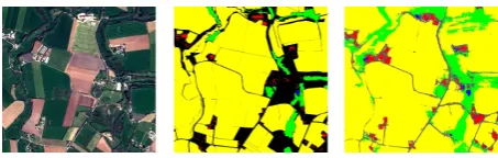
clas-Figure 1. Coverage of the training data. From left to right: Spot 6 image, training data, classification.●no training data,●
buildings,●roads,●crops,●forest,●water.
sification (Farabet et al., 2013). State-of-the-art algorithms fol-low the principle that the deeper the neural networks, the more specific and discriminant the information one may extract from images (Simonyan and Zisserman, 2014; Szegedy et al., 2015). However, increasing the depth of the networks also leads to a larger number of parameters and this may result into overfitting especially when training data are not sufficiently abundant1. In order to mitigate this problem, several techniques have been de-veloped, such as augmenting training sets, dropout (Srivastava et al., 2014) or batch normalization (Ioffe and Szegedy, 2015).
In the particular context of LC mapping, existing DCNN solu-tions achieve classification at different levels; on the one hand, patch-based approaches (see for instance (Girshick et al., 2014)) estimate, for each region centered on a pixel, a vector of proba-bility distribution, describing the membership of that region to different classes. On the other hand, dense approaches (such as (Long et al., 2015)) may learn pixel-based structure through deconvolution layers and are suitable in order to accurately de-limit the boundaries of objects of interest. The approach pre-sented in this paper is a patch-based one; it investigates the poten-tial of DCNNs for operational patch-based land-cover mapping at the country scale, using monoscopic VHR satellite imagery (namely, SPOT 6 and SPOT 7 sensors with four spectral bands) and involving a small number of topographic LC classes. Such imagery can be captured yearly at the country scale and may be used to monitor changes. In very recent years, various works have already shown the efficiency of deep architectures for semantic segmentation of geospatial VHR images (see for instance (Mar-manis et al., 2016a,b; Paisitkriangkrai et al., 2016; Maggiori et al., 2017; Volpi and Tuia, 2017). However, they remain at an experimental level, they also focus on sharp class boundary de-tection and require data that may not be available/updated yearly at large scales (i.e., Digital Surface Models and/or sub-meter spa-tial resolution images). Our study only relies on monoscopic and mono-temporal imagery, on existing land-cover maps, fed into a simple yet efficient architecture, that does not require out-of-standard computing capacities.
A short literature survey is first proposed in Section 2. The de-signed architecture and the experiments are presented in tions 3, and 4, respectively. Main outcomes are discussed in Sec-tion 5 and conclusions are drawn in SecSec-tion 6.
2. RELATED WORKS 2.1 Semantic classification
Semantic classification is a recurrent topic in remote sensing and computer vision communities. The adoption of DCNNs so as to
1
Overfitting is the effect that causes the parameters of a model to fit exactly the training data, leading to poor generalization capacity on un-seen data.
achieve such task correspond to most of the recent state-of-the-art literature. Farabet et al. (2013) perform a multi-scale analysis through CNNs, jointly used with superpixels built with a seg-mentation tree, to obtain a semantic segseg-mentation map of video frames.
A popular type of network emerged recently to tackle the problem of scene parsing differently from (Farabet et al., 2013); instead of using a segmentation tree, local spatial arrangements are learned withfully convolutional networks(FCN) (Long et al., 2015). The trick of such networks consists in considering the fully connected layers at the top of a neural net as convolutional ones, providing coarse probability maps as outputs instead of a probability vec-tor. These heat maps are then upsampled to the input image size through learned upsampling layers calleddeconvolutionlayers. Successive teams used that encoder-decoder frame to design task-specific architectures after its impressive success on the PASCAL VOC2012 (Everingham et al., 2012). SegNet (Badrinarayanan et al., 2015) improved the object delineation by mitigating the loss of information during the pooling process in the encoder part, thanks to connections from these very pooling layers to the corre-sponding deconvolution layers in the decoder part. Alternatively, the ResNet architecture (He et al., 2016) has become very pop-ular by challenging the assumption that each layer only needs information from the previous layer, and thus improving results on ImageNet and COCO 2015 detection and segmentation chal-lenges.
FCN-based architectures have become a standard for semantic classification but preferably require dense training data (parti-tion of the training image patches), unlike patch-based methods that only require a single label per training patch. Such training dataset is hard to obtain when not using benchmark datasets. In the context of this study, country-scale land-cover geodatabases are available but do not propose a dense partition of the Earth sur-face as shown in Fig. 1. Hence, a patch-based approach should be adopted here, also to ensure a same amount a samples for each class, avoiding an unbalanced training set.
2.2 Scene parsing in overhead imagery
The remote sensing community recently got interested in deep learning methods for land-cover mapping. Overhead imagery, especially VHR geospatial imagery, proposes classification chal-lenges, both in terms of accuracy and scalability. Compared to standard classifiers using hand-crafted features, DCNNs scale ef-ficiently with the diversity of appearances for a given class by training over all possible representations of a class.
Figure 2. Proposed architectures: the 3-l CNN is represented, the 4-l has a similar scheme with a 4th convolutional and
pooling layer.
state-of-the-art accuracy. Sherrah (2016) also fed both DSM and aerial imagery to a custom FCN denoted as no-downsampling FCN. By using the ”a trous” algorithm first used in CNNs by (Chen et al., 2014), they removed the pooling layers that caused the downsampling effect by construction, thereby preserving the input size. They achieve one of the best results on the ISPRS Vai-hingen and Potsdam datasets.
Audebert et al. (2016) integrated multi-kernel convolutional layers in the decoder part of the SegNet architecture (Badri-narayanan et al., 2015) to capture multi-scale information while upsampling. They also introduced the fusion network to deal with both DSM and images: they are first separately fed to two Seg-Net, whose outputs are concatenated and fed to a 3-convolution layers network.
Volpi and Tuia (2017) also achieve state-of-the-art results on the ISPRS Vaihingen and Potsdam datasets with their full patch la-beling architecture. It consists in a FCN with a 3x3 deconvolu-tion layer, that replaces the fully-connected layers in ”tradideconvolu-tional” CNNs. Additionally, a computational comparison between FCN and patch-based approaches shows that, although the training time is longer for the first, the inference time is a lot faster be-cause the prediction is directly made for all the pixels within the patch. On the contrary, the patch-based approach predicts a label for a single pixel. Recently, efforts have been made for joint edge detection and semantic classification (Marmanis et al., 2016b).
Hu et al. (2015) investigate the relevance of using DCNNs from the state-of-the-art in object detection and recognition for over-head scene classification. To do so, they focused on extracting features from those CNNs features at different layers and used them to label images from two datasets: UC Merced Dataset (UCM) (Yang and Newsam, 2010) and the WHU-RS Dataset (Xia et al., 2010). These datasets contain a single label per im-age, unlike previous papers which needed dense labeling, as men-tioned in the introduction. The authors could boost classification accuracies respectively by 2.5% and 5%, pointing out the useful-ness of state-of-the-art CNNs features for overhead scene clas-sification. Penatti et al. (2015) led the same study on the UCM dataset and got to the same conclusion as previously.
The present work is related to the two latter approaches. The reason first lies in the available training dataset: non-dense la-bels stemming from existing land-cover databases prevent from performing similar work as Sherrah (2016). Secondly, for many operational tasks such as database verification, updating, or statis-tics retrieval, the accurate delineation of objects may not appear to be necessary.
3. METHOD
In this part, the two main components of the processing chain are described. First, the two tested CNNs are presented. The purpose is to evaluate the impact of the number of layers on the output. Secondly, the creation of the training dataset is described. Indeed, as mentioned above, it is proposed to use the richness of available
geodatabases to build the training set. Since no dataset the com-munity is accustomed to is used here, this aspect of this work is emphasized.
All experiments are computed on a standard desktop machine with the following setup: an Intel Core i7-4790/8 Gb RAM for the CPU part, and an Nvidia GeForce GTX 980 / 4 Gb RAM for the GPU part.
3.1 CNN architectures
Lots of work have already been done in the FCN field for remote sensing applications (Section 2) but this type of architecture re-quires heavy tuning, in particular for the upsampling part, and has a strong condition on the training set. Thus, a patch-based approach was chosen. Another specificity of the proposed frame-work lies in the fact that it has to be light, so it can be computed on light desktop machines such as the one described above. Fi-nally, the architecture needs not only to be light, but also able to label very large regions at a 1.5m resolution in reasonable time. Regarding the size of input patches of the nets, a trade-off had to be made. The classification is meant to be territory-exhaustive re-quiring to deal with objects of different spatial extent: small-sized classes such as buildings or roads and large-sized ones such as forests, crop fields and water areas. Thus, a 65x65x4 input patch size was adopted for every classes so that small objects were well enough represented. Although linear objects such as roads and rivers can occur, no particulara prioriwas made, (i) in order to remain task-generic, (ii) because the object structure is caught by the neighborhood within the patch. All available spectral bands, namelyRed (R), Green (G), Blue (B), Infra-Red (IR), were used.
CNNs are successions of convolutional layers, themselves made of several trainable filters. Each filter is followed by a non-linear function to account for the fact that the final model of data is non-linear. The filters weights are shared through the image to avoid a huge increase of the parameters. On top of it, a classifier will deliver the desired output by minimizing a loss function. Two light architectures were designed, differing only by their number of layers: a 3-layer network and a 4-layer network were built. The first net is illustrated in Fig. 2. They will be further referred as 3-l and 4-l respectively. Each convolutional layer is followed by a 2x2-pooling layer to: (i) introduce small transla-tion invariance, (ii) increase the receptive field of neurons with the depth of the net, inducing a multi-scale analysis, (iii) only preserve meaningful spatial information. Pooling enables to de-tect objects independently on their location on the image. In this way, an isolated house in the countryside has as good odds to be detected as a house in a dense urban area. Such property is vital to detect buildings independently on their location on images for instance.
The ”non-linearity” function chosen is the well-known Rectified Linear Unit (ReLU) introduced first by (Nair and Hinton, 2010), which improves training by mitigating the vanishing gradient that other functions induce due to their saturating property.
On top of all these layers, one fully-connected layer is in-tegrated, followed by the largely used cross-entropy criterion, whose scores are provided by asoftmaxlayer.
The CNN bindings are provided by the Torch library2.
3.2 Building the training dataset
The training datasets are built upon national reference topo-graphic geodatabases as shown on Fig. 1. These geodatabases
2
Figure 3. Comparison of 3-l (middle) and 4-l nets (right): the reference data is on the left.
containing lots of vector data as well as raster data (Spot 6 and Spot 7 images) are georeferenced and perfectly overlap. The ac-curacy of the databases is 1m, which is compatible with the 1.5m resolution of the images: any geometric error in the geodatabase is inferior to 1m, causing only errors inferior to the pixel in the final classification. Nonetheless, the geodatabases are not neces-sarily up-to-date everywhere: buildings can be built where a for-est was standing when the information within the geodatabases were gathered. In general, such errors are very rare because the databases are regularly updated by human operators. With this in mind, it appears that using CNNs is relevant for this task. Even with noisy labels, CNNs can hopefully behave as expected when fed with substantial amounts of training data.
A protocol was defined to select 65×65×4 training sample patches. For each class, a regular sampling of training points is performed over the whole training area. These points are then turned to training patches by selecting their respective65×65 neighborhood. 10,000 samples were selected per class, with 10% kept for validation.
During training, online data transformations are randomly per-formed, not only so as to mitigate overfitting, but also to force the system to learn invariances. For instance, overhead imagery can be acquired at random azimuth, meaning that the features need to be rotation invariant.
3.3 Training the CNNs
The 3-l and 4-l nets are trained from the dataset build as described above on a chosen area (see Section 4.1 for further details on the regions of interest in this work). Two strategies were investigated for this step: a Random Weights Initialization (RWI), and Fine-Tuned Nets (FTN) previously pre-trained with random weight initialization. In practice, mini-batches of size 200 were used during all training steps. As mentioned above, an online random data augmentation is also performed on each mini-batch.
3.3.1 Random Weight Initialization (RWI) At our knowl-edge, there is no light pre-trained network available with RGB-IR data. Hence training was here performed with random parame-ters as initialization. It was run during 5,000 epochs, for all tests with RWI. The reason for such a large number of iterations lies in the fact that we had no insight of the required number of epochs before reaching a suitable convergence limit.
3.3.2 Fine-Tuned Net (FTN) A pre-trained state-of-the-art net has the advantage to offer a potentially already well-tuned very deep network. However, such nets (Simonyan and Zisser-man, 2014; Szegedy et al., 2015) are very sensitive to the nu-merous hyper-parameters to set, and require specific work to find optimal configurations, and to actually train them.
The process is the same as for RWI except for the initialization: it consists in learning specific characteristics of a new training dataset with a net already pre-trained (with RWI) on another dataset. In computer vision, it proved to be more efficient than
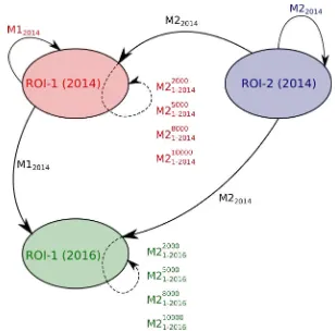
Figure 4. Experiments during training with both methods described in Section 3 (dotted lines: FTNs on the new area) ROI-1(2014), ROI-1(2016), ROI-2(2014) stand for the Spot images acquired on Brest in 2014/2016 and Le Faou in 2014.
RWI, but this can be tedious due to the number of parameters to optimize. In particular, various works only fine-tuned the last convolutional layers. Indeed, the first layers of CNNs mostly de-scribe low-level image features, such as edges (Zeiler and Fer-gus, 2014). This type of features can be stated as common to all computer vision tasks: edges are the lowest level of information one would retrieve from the image. On the opposite, the deep-est layers are more task-specific: these are the ones that would be fine-tuned, while the shallower ones are frozen, reducing the number of parameters to re-estimate.
In this work,fine-tuning is applied on our networks(Fig. 2). Due to the pre-trained aspect of the net used for fine-tuning, few iterations are necessary to converge compared to the RWI strat-egy, making FTN faster and even more interesting. When using FTN, the training is run up to 300 epochs. Several FTN have been produced with different amount of new training data to study the impact it has on the output quality.
3.4 Inference
At test time, since a patch-based approach was chosen, the se-mantic classification is produced by sliding a window over the image to label. The window is centered on each pixel and has the size of the net input, that is to say 65×65×4. The label assigned to the current pixel is the output label returned by the net when forwarding the window centered on this very pixel. In order to track the results for very large geographic areas, and avoid loss of information in case of a system error, the image to label (up to 50 GB for a unique image) is tiled to 2,000×2,000 images.
4. EXPERIMENTS
All experiments here aim at labeling the images into five different classes:building, road network, forests, crops, water. As shown in Section 5, such a reduced classification for large scale applica-tions has strong limitaapplica-tions.
but also challenging if one tries to generate a model on one of these two areas, and to test it on the other one. In addition to the different geographic situation of the areas, two different dates of acquisition on these areas are studied (2014 and 2016).
4.2 Experiments
In this work, studying different strategies for training is vital to be able to produce large scale semantic segmentation. Thus, several experiments have been led at training level. Fig. 4 shows the strategies explored in this study.
4.2.1 Training nets with RWI Training datasets have been built following the method in Section 3, on both ROI-1 (2014) and ROI-2 (2014). RWI nets are the shared foundation of all ex-periments, since no pre-trained network with RGB-IR channels was available. 4-l nets have been trained with RWI, and tested on both regions with the patch-based approach described above. These experiments are designated respectively as M12014 and
M22014respectively on Fig. 4. M12014 also encapsulates the
only training and test made with 3-l, in order to assess the impact of the depth of the net. This whole part focuses on the raw con-sistency of a net so as to generalize over unseen regions without further tuning.
4.2.2 FTNs across geographic and ”time” areas
a. Fine-tuninghas been investigating for two reasons: (i) reduc-ing computation times, (ii) learn specificities of new areas while preserving those of previous areas. Indeed, training a net with RWI on ROI-2 will produce features that would capture the geo-metric particularities of rural regions. At test time, this trained net would be expected to perform poorly on ROI-1, which is mostly dense urban area. Fine-tuning comes up as an interest-ing choice to improve the generalization capacity of the network trained on ROI-1. The influence of the size of the training dataset is also gauged when fine-tuning. FTNs on Fig. 4 are designated asM Nxxxx
P−year, whereN andP are ROI identifications desig-nated the ROIs where the pre-trained network and the fine-tuned net respectively come from,yearthe year of the image acquisi-tion where lies ROIP andxxxxthe amount of training samples coming from ROIP.
b. Generalization capacity across geographic areasis natu-ral to look into for this task. However, land-cover raises strong interests inchange detection. This induces a need to compare thesame region at different dates. Vegetation appearances, dif-ferences in crop growths bring huge disparities in the spectrum for a given class. ROI-1 (2016) is the test led on the image on ROI-1 acquired in 2016. First,M12014has been tested on ROI-1
(2016), then the net trained on ROI-2 (2014) was fine-tuned over ROI-1 (2016) as well. These latter experiments (with different amounts of training data) aim at evaluating the capacity to be-have correctly, for a net first pre-trained on aruralarea, but also at an interval of two years (time consistency of a net).
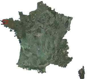
4.2.3 Prediction across large area The problematic being the semantic classification of country scale regions, a predic-tion was performed over a sub-region representing 26% of the Finist`ere, or 1,755 km2
(ROI-3) which has been labeled with M12014. The fact that no re-adjustment of this net has been
done should be underlined, yet this case of study is difficult. In-deed, ROI-3 is a region which is mostly rural, andM12014 is
a net trained over a dense urban area (Brest). Furthermore, LC labels are very varying in appearance compared to the patches
Figure 5. SPOT 6/7 coverage of France in 2014 - Red frame is ROI-3.
representing the same LC labels in the training dataset used for M12014. In particular, new types of water areas, such as
estuar-ies, and moor lands (typical of French Brittany) are present in the test image, but were not learned byM12014. The footprint of the
labeled area can be seen on Fig. 5.
5. RESULTS 5.1 Quality assessment
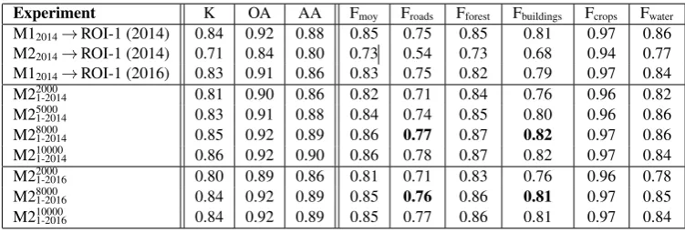
Results were evaluated by comparing the semantic classification to a ground truth derived from the geodatabases (Fig. 1). Geo-database objects were eroded by one pixel to leave the possi-ble uncertainties on object edges. A pixel-to-pixel comparison gives confusion matrices from which are derived several mea-sures. Two of these measures are whether, class-specific, namely the average accuracy (AA) and the average F1 score (Fmoy). The AA is the ratio of correctly labeled pixels for a given class. The F1-score is the ratio of precision (well-classified pixel for the given class) and recall (missing pixels in the given class). The other two measures, Kappa (K) and the overall accuracy (OA), give global qualities, thus are sensitive to the difference in size of the classes. OA is the rate of well-classified pixels while K takes into account the random composite during labeling.
At each experiment, the final classification did not undergo any further adjustment such as Conditional Random Fields (CRF). The absence of refinement thus impacts the quality assessment since it is a pixel-to-pixel evaluation (remaining noise). Water class is also assessed though it is often hard to evaluate it effi-ciently due to (i) the diversity of this class representation (bonds in quarries, natural bonds, estuaries, sea) (ii) the shadows that of-ten pollute the quality by being mislabeled aswater.
An evaluation of the generalization capability of neural nets for our goal was also led with the experiment on ROI-3. By strati-fying the qualification along the 2,000×2,000 tiles used for pre-diction as mentioned in Section 3, the performance of the model learned on ROI-1 (2014) can be assessed when geographically moving away from the initial training area.
5.2 Training nets with RWI and direct feed-forward for pre-diction
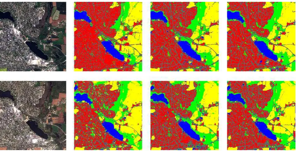
Figure 6. Illustration of the changes of the learning strategies over a small part of ROI-1. Top row: 2014 data. From left to right: 2014 image,M22014,M2
2000 1
−2014,M2
8000 1
−2014. Bottom row: 2016 data. From left to right: 2016 image,M12014,M2
2000 1
−2016,M2
8000 1
−2014.
epochs were necessary in both cases. Fine-tuning, on the other hand, was only performed on the 4-l type of net since it always showed the best results on every experiments were both 3-l and 4-l were assessed. Fig. 3 puts together results from a 3-l net pre-diction and a 4-l net prepre-diction over the same area, the ground truth is also provided for visual appreciation.
The three first rows of Table 1 detail the results on the training part with RWI net. The first line corresponds to a RWI net trained on data selected on ROI-1(2014) and then applied to the same ROI: roads and buildings are surprisingly well classified, with accuracies that have never been reached before. Crop class has a very good F1-score, which happens generally due to the amount of crop pixel both in the ground truth and the semantic classifica-tion (errors are drown into the mass of correctly classified pixels). Secondly comes the net model trained on ROI-2 then applied to ROI-1 (2014): a drop in all measures can be noticed. The di-versity in the type of classes present in both regions, especially because ROI-1 is densely urban while ROI-2 is mostly country-side, has an impact on Fbuildingand Froad, which are the most im-pacted. Finally, the net trained on ROI-1 (2014) was tested on ROI-1 (2016) to answer the interrogation about time consistency. A slight decrease of the quality is shown, but remaining strongly close to the quality of the 2014 results on the same area. A valu-able property of time consistencyof the net is thus to be under-lined. The two latter results can be visualized on Fig. 6. For such light architectures, results are in general promising with RWI nets. In particular, the roads and buildings retrieved by the classifier are very satisfying, even in dense urban areas. Road detection was a topic studied by Mnih and Hinton (2010) who designed a specific semi-supervised method. The semantic clas-sification over VHR images also offers a land-cover with accurate object delineation in urban areas, even without the use of a DSM as in previous works, or any shape or radiometric a priori.
5.3 Fine-tuning of pre-trained net by RWI
We focused on the ROI-1 for these experiments to cope the am-biguities on the dense urban network that was not retrieved when
predicting with a net trained on another area. We also looked at the impact of the training set size used for fine-tuning. The fine-tuning steps ran up to 300 epochs, but 200-250 were needed before they reached an asymptotic maximum quality. Two main experiments have been led, furthering the work on the two last works discussed in the previous paragraph. Fine-tuning always acts on the pre-trained net (with RWI) on ROI-2(2014) and ap-plied to ROI-1.1. FTN to disambiguate urban areashas been studied by re-learning the 2 net with training data from ROI-1(2014). The four middle lines of Table 1 present the obtained results. A general improvement can be noticed, especially for roadandbuildingclasses with respective increases of 23% and 14% for the fine-tuned net with 8,000 samples/class. The impact of fine-tuning can be visually assessed on Fig. 6. This under-lines the geographic influence of the training samples selection: the RWI net was trained on a rural area with simple urban struc-ture, resulting in poor urban description on a dense area. This bottleneck is mitigated by injecting dense urban training samples during net re-training.
2. Predicting across time as well as on urban areasis an-other task addressed, by predicting on ROI-1 (2016) with the net trained on ROI-2 (2014). The qualities of the related tests are ex-posed on the three bottom lines of Table 1. Results that can be observed are also very satisfying as the amount of training data increases, and are similar to the first experiments on fine-tuning. Compared to the ROI-1 (2014) net applied on ROI-1 (2016) im-age, improvement is also observed, suggesting that the ability to handle time changing and urban description from a net not origi-nally designed for these tasks.
Figure 7. Land-cover produced on ROI-3 with a 4-l net trained on ROI-1 (2014). The size of ROI-3 is 39×45 km.
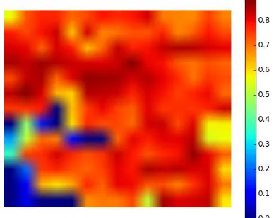
Figure 8. Kappa index obtained on ROI-3.
5.4 Large scale semantic classification
The large scale semantic classification was performed by sliding a window over ROI-3, which was tiled into 2,000×2,000 images. The resulting land-cover map can be seen on Fig. 7. Labeling such an area took 4 days on our standard desktop machine. The training area for the net is located around Brest (largest urban area, in red), and corresponds to about 8% to the labeled area. 780 millions of pixels have been labeled this way. Along the vi-sual product, Fig. 8 shows the the kappa index as a heat map. Each pixel of these maps correspond to a 2,000×2,000 tile, al-lowing geographic analysis of the quality. Some blue pixels on the heat maps seem to indicate poor classification on the corsponding regions, but comparing to Fig. 7 reveals that these re-gions are whether coastal or maritime.
This large scale land-cover with a very light architecture already retrieve the main regions on ROI-3. Rural regions have a slight decrease in quality due to the training dataset that was made on a dense urban area, thus less efficient on natural areas. Estuar-ies are also mislabeled as building instead of water due to their particular appearance (texture).
6. CONCLUSIONS AND PERSPECTIVES
A light architecture was designed and trained according to dif-ferent strategies, so as to perform a large scale semantic classifi-cation over VHR satellite images. Constrained by the geograph-ically sparse reference data, the patch-based approach was se-lected. Although it prevents from a fine description of pixel-level spatial arrangement, it is easier to train (absence of deconvolution layers), and it shows very promising results. RWI nets already bring a fine delineation of objects, but also show satisfying ur-ban description. In particular, theroad networkgets good results when it comes to labeling dense urban areas with nets trained on similar type of region, and this was done without any particular a priori. Indeed, it is important to note that every classes were processed in the same manner, at training samples selection and at training time. Drops in measures appear when the net predicts labels on another geographic area. Cropsandforestsclasses, on the other hand, also show very high performances, in most cases, with ambiguities that occur when crops have strong resembling textures with forests, that were not learned by the net. An in-teresting result is that RWI strategy also proves to be insensitive to time changing when labeling the same region at two different dates, which is positive in a change detection context.
In order to cope with these ambiguities, the nets pre-trained with RWI were fine-tuned, with several amounts of training data from the unseen region. Increasing the number of samples to fine-tune nets improve the results, although quality reach its limit around 8,000 samples/class. Theroad networkandbuildingclasses get substantial improvement. Such improvements suggest that there is a geographic dependency of the net during training (dense or sparse urban area, type of vegetation).
One can eventually note the very satisfactory discrimination re-sults at large scale, despite (i) a very restricted training set in terms of spatial extent and (ii) the diversity of the classes of in-terest in terms of appearance.
Future work will focus on increasing the number of classes, jointly with the use of Sentinel-2 time series in order to retrieve (i) classes that were mixed in theforestclass, leading to mislabel-ing, and (ii) to diversify thecropclass. The produced large scale land-cover map covers a part that is very rich in terms of types of vegetation. We could observe issues, in particular, on coastal moor lands, very frequent in this territory. Also, confusions be-tweenhedgesandroadsappeared, suggesting there again a new class to consider. In addition, hard training is planned to force the net to learn from difficult samples.
References
Audebert, N., Le Saux, B. and Lef`evre, S., 2016. Semantic segmentation of earth observation data using multimodal and multi-scale deep networks. In:ACCV.
Badrinarayanan, V., Kendall, A. and Cipolla, R., 2015. Segnet: A deep convolutional encoder-decoder architecture for image segmentation.arXiv:1511.00561.
Chen, L.-C., Papandreou, G., Kokkinos, I., Murphy, K. and Yuille, A. L., 2014. Semantic image segmentation with deep convolutional nets and fully connected CRFs. arXiv:1412.7062.
Experiment K OA AA Fmoy Froads Fforest Fbuildings Fcrops Fwater M12014→ROI-1 (2014) 0.84 0.92 0.88 0.85 0.75 0.85 0.81 0.97 0.86 M22014→ROI-1 (2014) 0.71 0.84 0.80 0.73 0.54 0.73 0.68 0.94 0.77 M12014→ROI-1 (2016) 0.83 0.91 0.86 0.83 0.75 0.82 0.79 0.97 0.84
M21-20142000 0.81 0.90 0.86 0.82 0.71 0.84 0.76 0.96 0.82
M21-20145000 0.83 0.91 0.88 0.84 0.74 0.85 0.80 0.96 0.86
M21-20148000 0.85 0.92 0.89 0.86 0.77 0.87 0.82 0.97 0.86
M21-201410000 0.86 0.92 0.90 0.86 0.78 0.87 0.82 0.97 0.84
M21-20162000 0.80 0.89 0.86 0.81 0.71 0.83 0.76 0.96 0.78
M21-20168000 0.84 0.92 0.89 0.85 0.76 0.86 0.81 0.97 0.85
M21-201610000 0.84 0.92 0.89 0.85 0.77 0.86 0.81 0.97 0.84
Table 1. Assessment of the training and testing schemes designed in this work.
Farabet, C., Couprie, C., Najman, L. and LeCun, Y., 2013. Learn-ing hierarchical features for scene labelLearn-ing.IEEE Transactions on Pattern Analysis and Machine Intelligence35(8), pp. 1915– 1929.
Gerke, M., 2014. Use of the Stair Vision Library within the IS-PRS 2D semantic labeling benchmark (Vaihingen). Technical report, ITC, University of Twente, The Nederlands.
Girshick, R., Donahue, J., Darrell, T. and Malik, J., 2014. Rich feature hierarchies for accurate object detection and semantic segmentation. In:CVPR, pp. 580–587.
Gressin, A., Mallet, C., Vincent, N. and Paparoditis, N., 2013. Updating land cover databases using a single very high resolu-tion satellite image.ISPRS Annals of Photogrammetry, Remote Sensing and Spatial Information SciencesII-3/W2, pp. 13–18.
Gressin, A., Vincent, N., Mallet, C. and Paparoditis, N., 2014. A unified framework for land-cover database update and enrich-ment using satellite imagery. In:IEEE ICIP, pp. 5057–5061.
He, K., Zhang, X., Ren, S. and Sun, J., 2016. Deep residual learning for image recognition. In:CVPR, pp. 770–778.
Hu, F., Xia, G.-S., Hu, J. and Zhang, L., 2015. Transferring deep convolutional neural networks for the scene classification of high-resolution remote sensing imagery. Remote Sensing 7(11), pp. 14680–14707.
Ioffe, S. and Szegedy, C., 2015. Batch normalization: Accelerat-ing deep network trainAccelerat-ing by reducAccelerat-ing internal covariate shift. arXiv:1502.03167.
Jia, K., Liang, S., Wei, X., Zhang, L., Yao, Y. and Gao, S., 2014. Automatic land-cover update approach integrating it-erative training sample selection and a Markov random field model.Remote Sensing Letters5(2), pp. 148–156.
Khatami, R., Mountrakis, G. and Stehman, S., 2016. A meta-analysis of remote sensing research on supervised pixel-based land-cover image classification processes: General guidelines for practitioners and future research. Remote Sensing of Envi-ronment177, pp. 89–100.
Krizhevsky, A., Sutskever, I. and Hinton, G. E., 2012. Ima-genet classification with deep convolutional neural networks. In:NIPS, pp. 1097–1105.
Long, J., Shelhamer, E. and Darrell, T., 2015. Fully convolutional networks for semantic segmentation. In: CVPR, pp. 3431– 3440.
Maas, A., Rottensteiner, F. and Heipke, C., 2016. Using label noise robust logistic regression for automated updating of to-pographic geospatial databases. ISPRS Annals of Photogram-metry, Remote Sensing and Spatial Information SciencesIII-7, pp. 133–140.
Maggiori, E., Tarabalka, Y., Charpiat, G. and Alliez, P., 2017. Convolutional neural networks for large-scale remote-sensing image classification.IEEE TGRS55(2), pp. 645–657.
Marmanis, D., Schindler, K., Wegner, J., Galliani, S., Datcu, M. and Stilla, U., 2016a. Classification with an edge: Im-proving semantic image segmentation with boundary detec-tion.arXiv:1612.01337.
Marmanis, D., Wegner, J., Galliani, S., Schindler, K., Datcu, M. and Stilla, U., 2016b. Semantic segmentation of aerial images with an ensemble of fully convolutional neural networks. IS-PRS Annals of Photogrammetry, Remote Sensing and Spatial Information SciencesIII-3, pp. 473–480.
Mnih, V. and Hinton, G. E., 2010. Learning to detect roads in high-resolution aerial images. In:ECCV, pp. 210–223.
Nair, V. and Hinton, G. E., 2010. Rectified linear units improve restricted Boltzmann machines. In:ICML, pp. 807–814.
Paisitkriangkrai, S., Sherrah, J., Janney, P. and Hengel, A. V. D., 2016. Semantic labeling of aerial and satellite imagery. IEEE JSTARS9(7), pp. 2868–2881.
Penatti, O., Nogueira, K. and dos Santos, J. A., 2015. Do deep features generalize from everyday objects to remote sensing and aerial scenes domains? In:IEEE CVPR Workshops, Earth-vision.
Sherrah, J., 2016. Fully convolutional networks for dense semantic labelling of high-resolution aerial imagery. arxiv:1606.02585.
Simonyan, K. and Zisserman, A., 2014. Very deep convolutional networks for large-scale image recognition.arXiv:1409.1556.
Srivastava, N., Hinton, G. E., Krizhevsky, A., Sutskever, I. and Salakhutdinov, R., 2014. Dropout: a simple way to prevent neural networks from overfitting.JMLR15(1), pp. 1929–1958.
Szegedy, C., Liu, W., Jia, Y., Sermanet, P., Reed, S., Anguelov, D., Erhan, D., Vanhoucke, V. and Rabinovich, A., 2015. Going deeper with convolutions. In:CVPR, pp. 1–9.
Tokarczyk, P., Wegner, J. D., Walk, S. and Schindler, K., 2015. Features, color spaces, and boosting: New insights on semantic classification of remote sensing images. IEEE TGRS53(1), pp. 280–295.
Volpi, M. and Tuia, D., 2017. Dense semantic labeling of sub-decimeter resolution images with convolutional neural net-works.IEEE TGRS55(2), pp. 881–893.
Xia, G.-S., Yang, W., Delon, J., Gousseau, Y., Sun, H. and Maˆıtre, H., 2010. Structural high-resolution satellite image indexing. ISPRS Archives of Photogrammetry, Remote Sensing and Spa-tial Information ScienceXXXVIII-7A, pp. 298–303.
Yang, Y. and Newsam, S., 2010. Bag-of-visual-words and spatial extensions for land-use classification. In: ACM SIGSPATIAL, pp. 270–279.