SEMANTIC 3D SCENE INTERPRETATION: A FRAMEWORK COMBINING OPTIMAL
NEIGHBORHOOD SIZE SELECTION WITH RELEVANT FEATURES
Martin Weinmanna, Boris Jutzia, Cl´ement Malletb
a
Institute of Photogrammetry and Remote Sensing, Karlsruhe Institute of Technology (KIT) Englerstr. 7, 76131 Karlsruhe, Germany -{martin.weinmann, boris.jutzi}@kit.edu
b
IGN, MATIS lab., Universit´e Paris Est
73 avenue de Paris, 94160 Saint-Mand´e, France - [email protected]
Commission III, WG III/2
KEY WORDS:LIDAR, Point Cloud, Neighborhood Size Selection, Features, Feature Selection, Classification, Interpretation
ABSTRACT:
3D scene analysis by automatically assigning 3D points a semantic label has become an issue of major interest in recent years. Whereas the tasks of feature extraction and classification have been in the focus of research, the idea of using only relevant and more distinctive features extracted from optimal 3D neighborhoods has only rarely been addressed in 3D lidar data processing. In this paper, we focus on the interleaved issue of extracting relevant, but not redundant features and increasing their distinctiveness by considering the respective optimal 3D neighborhood of each individual 3D point. We present a new, fully automatic and versatile framework consisting of four successive steps: (i) optimal neighborhood size selection, (ii) feature extraction, (iii) feature selection, and (iv) classification. In a detailed evaluation which involves5different neighborhood definitions,21features,6approaches for feature subset selection and2 different classifiers, we demonstrate that optimal neighborhoods for individual 3D points significantly improve the results of scene interpretation and that the selection of adequate feature subsets may even further increase the quality of the derived results.
1 INTRODUCTION
The automatic interpretation of 3D point clouds represents a fun-damental issue in photogrammetry, remote sensing and computer vision. Nowadays, different subtopics are in the focus of research such as point cloud classification (Hu et al., 2013; Niemeyer et al., 2014; Xu et al., 2014), object recognition (Pu et al., 2011; Velizhev et al., 2012), creation of large-scale city models (La-farge and Mallet, 2012) or urban accessibility analysis (Serna and Marcotegui, 2013). For all of them, it is important to cope with the complexity of 3D scenes caused by the irregular sampling and very different types of objects as well as the computational burden arising from both large 3D point clouds and a variety of available features.
For scene interpretation in terms of uniquely assigning each 3D point a semantic label (e.g. ground,buildingorvegetation), the straightforward approach is to extract respective geometric fea-tures from its local 3D structure. Thus, the feafea-tures rely on a local 3D neighborhood which is typically chosen as spherical neighborhood with fixed radius (Lee and Schenk, 2002), cylin-drical neighborhood with fixed radius (Filin and Pfeifer, 2005) or spherical neighborhood formed by a fixed number of thek closest 3D points (Linsen and Prautzsch, 2001). Once features have been calculated, the classification of each 3D point may be conducted via standard supervised learning approaches such as Gaussian Mixture Models (Lalonde et al., 2005), Support Vec-tor Machines (Secord and Zakhor, 2007), AdaBoost (Lodha et al., 2007), a cascade of binary classifiers (Carlberg et al., 2009), Random Forests (Chehata et al., 2009) and Bayesian Discrimi-nant Classifiers (Khoshelham and Oude Elberink, 2012). In con-trast, contextual learning approaches also involve relationships among 3D points in a local neighborhood1which have to be in-ferred from the training data. Respective methods for classifying
1This local neighborhood is typically different from the one used for
feature extraction.
Figure 1: 3D point cloud with assigned labels (wire: blue, pole/trunk: red, fac¸ade: gray, ground: brown, vegetation: green).
point cloud data have been proposed with Associative and non-Associative Markov Networks (Munoz et al., 2009a; Shapovalov et al., 2010), Conditional Random Fields (Niemeyer et al., 2012), multi-stage inference procedures focusing on point cloud statis-tics and relational information over different scales (Xiong et al., 2011), and spatial inference machines modeling mid- and long-range dependencies inherent in the data (Shapovalov et al., 2013).
Since the semantic labels of nearby 3D points tend to be cor-related (Figure 1), involving a smooth labeling is often desir-able. However, exact inference is computationally intractable when applying contextual learning approaches. Instead, either approximate inference techniques or smoothing techniques are commonly applied. Approximate inference techniques remain challenging as there is no indication towards an optimal inference strategy, and they quickly reach their limitations if the considered neighborhood is becoming too large. In contrast, smoothing tech-niques may provide a significant improvement concerning classi-fication accuracy (Schindler, 2012). All of these techniques ex-ploit either the estimated probability of a 3D point belonging to each of the defined classes or the direct assignment of the respec-tive label, and thus the results of a classification for individual 3D points. Consequently, it seems desirable to investigate sources for potential improvements with respect to classification accuracy.
pa-rameterization of the neighborhood is still typically selected with respect to empirical a priori knowledge on the scene and identi-cal for all 3D points. This raises the question about estimating the optimal neighborhood for each individual 3D point and thus increasing the distinctiveness of derived features. Respective ap-proaches addressing this issue are based on local surface variation (Pauly et al., 2003; Belton and Lichti, 2006), iterative schemes relating neighborhood size to curvature, point density and noise of normal estimation (Mitra and Nguyen, 2003; Lalonde et al., 2005), or dimensionality-based scale selection (Demantk´e et al., 2011). Instead of mainly focusing on optimal neighborhoods, fur-ther approaches extract features based on different entities such as points and regions (Xiong et al., 2011; Xu et al., 2014). Al-ternatively, it would be possible to calculate features at different scales and later use a training procedure to define which com-bination of scales allows the best separation of different classes (Brodu and Lague, 2012).
Considering the variety of features which have been proposed for classifying 3D points, it may further be expected that there are more and less suitable features among them. For compensating lack of knowledge, however, often all extracted features are in-cluded in the classification process, and a respective feature se-lection has only rarely been applied in 3D point cloud process-ing. The main idea of such a feature selection is to improve the classification accuracy while simultaneously reducing both com-putational effort and memory consumption (Guyon and Elisseeff, 2003; Liu et al., 2010). Respective approaches allow to assess the relevance/importance of single features, rank them according to their relevance and select a subset of the best-ranked features (Chehata et al., 2009; Mallet et al., 2011; Khoshelham and Oude Elberink, 2012; Weinmann et al., 2013).
In this paper, we use state-of-the-art approaches for classifying 3D points and focus on the interleaved issue of deriving an op-timal subset of relevant, but not redundant, features extracted from individual neighborhoods with optimal size. In compari-son to seminal work addressing optimal neighborhood size selec-tion (Pauly et al., 2003; Mitra and Nguyen, 2003; Demantk´e et al., 2011), we directly assess the order/disorder of 3D points in the local neighborhood from the eigenvalues of the 3D structure tensor. In comparison to recent work on feature selection for 3D lidar data processing (Mallet et al., 2011; Weinmann et al., 2013), we exploit entropy-based measures for (i) determining the opti-mal neighborhood size for each 3D point and (ii) removing irrele-vant and redundant features in order to derive an adequate feature subset. Both of these issues are crucial for the whole processing chain, and it is therefore of great importance to avoid parameters or thresholds which are explicitly selected by human interaction based on empiric or heuristic knowledge.
In summary, the main contribution of our work is a fully auto-matic versatile framework which is based on
• determining the optimal neighborhood size for each individ-ual 3D point by considering the order/disorder of 3D points within a covariance ellipsoid,
• extracting optimized 3D and 2D features from the derived optimal neighborhoods in order to optimally describe the lo-cal structure for each 3D point,
• selecting a compact and robust feature subset by address-ing different intrinsic properties of the given trainaddress-ing data via multivariate filter-based feature selection (based on both featuclass and featufeature relations) in order to re-move feature redundancy, and
• improving the classification accuracy by exploiting the de-rived feature subsets and state-of-the-art classifiers.
Our framework is generally applicable for interpreting 3D point cloud data acquired via airborne laser scanning (ALS), terrestrial laser scanning (TLS), mobile laser scanning (MLS), range imag-ing by 3D cameras or 3D reconstruction from images. While the selected feature subset may vary with respect to different datasets, the beneficial impact of both optimal neighborhood size selection and feature selection remains. Further extensions of the frame-work by involving additional features such as color/intensity or full-waveform features can easily be taken into account.
The paper is organized as follows. In Section 2, we explain the single components of our framework in detail. Subsequently, in Section 3, we evaluate the proposed methodology on MLS data acquired within an urban environment. The derived results are discussed in Section 4. Finally, in Section 5, concluding remarks are provided, and suggestions for future work are outlined.
2 METHODOLOGY
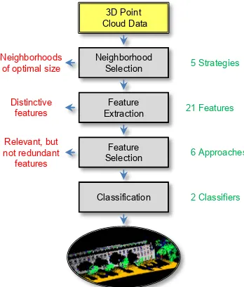
For semantically interpreting 3D point clouds, we propose a new methodology which involves neighborhood selection with opti-mal neighborhood size for each individual 3D point (Section 2.1), 3D and 2D feature extraction (Section 2.2), feature subset se-lection via feature-class and feature-feature correlation (Section 2.3), and supervised classification of 3D point cloud data (Sec-tion 2.4). A visual representa(Sec-tion of the whole framework and its components is provided in Figure 2.
3D Point Cloud Data
Neighborhood Selection
Feature Extraction
Feature Selection
Classification Neighborhoods
of optimal size
Distinctive features
Relevant, but not redundant features
5 Strategies
21 Features
6 Approaches
2 Classifiers
Figure 2: The proposed framework: the contributions are high-lighted in red, and the quantity of attributes/approaches used for evaluation is indicated in green.
2.1 Neighborhood Selection
In general, we may face a varying point density in the captured 3D point cloud data. Since we do not want to assume a priori knowledge on the scene, we exploit the spherical neighborhood definition based on a 3D point and itskclosest 3D points (Lin-sen and Prautzsch, 2001), which allows more flexibility with re-spect to the geometric size of the neighborhood. In order to avoid heuristically selecting a certain value for the parameterk, we fo-cus on automatically estimating the optimal value fork.
Assuming a point cloud formed by a total number ofN3D points and a given valuek ∈ N, we may consider each individual 3D pointX = (X, Y, Z)T ∈ R3
defining its scale. For describing the local 3D structure around X, the respective 3D covariance matrix also known as 3D struc-ture tensorS∈R3×3
is derived which is a symmetric positive-definite matrix. Thus, its three eigenvaluesλ1, λ2, λ3 ∈ R ex-ist, are non-negative and correspond to an orthogonal system of eigenvectors. Since there may not necessarily be a preferred vari-ation with respect to the eigenvectors, we consider the general case based on a structure tensor with rank3. Hence, it follows thatλ1≥λ2≥λ3≥0holds for each 3D pointX.
From the eigenvalues of the 3D structure tensor, the surface vari-ationCλ(i.e. the change of curvature) with
Cλ= λ3
λ1+λ2+λ3
(1)
can be estimated. For an increasing neighborhood size, the heuris-tic search for locations with significant increase ofCλallows to find the critical neighborhood size and thus to select a respec-tive value fork(Pauly et al., 2003). This procedure is motivated by the fact that occurring jumps indicate strong deviations in the normal direction. As alternative, it has been proposed to select the neighborhood size according to a consistent curvature level (Belton and Lichti, 2006).
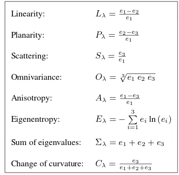
Further investigations focus on extracting the dimensionality fea-tures of linearityLλ, planarityPλand scatteringSλaccording to
Lλ= λ1−λ2
λ1
Pλ= λ2−λ3
λ1
Sλ= λ3
λ1
(2)
which represent 1D, 2D and 3D features. As these features sum up to1, they may be considered as the probabilities of a 3D point to be labeled as 1D, 2D or 3D structure (Demantk´e et al., 2011). Accordingly, a measureEdimof unpredictability given by the Shannon entropy (Shannon, 1948) as
Edim=−Lλln(Lλ)−Pλln(Pλ)−Sλln(Sλ) (3)
can be minimized across different scalesk to find the optimal neighborhood size which favors one dimensionality the most. For this purpose, the radius has been taken into account, and the inter-val[rmin, rmax]has been sampled in16scales, where the radii are not linearly increased since the radius of interest is usually closer tormin. The valuesrminandrmaxdepend on various characteris-tics of the given data and are therefore specific for each dataset. However, the results are based on the assumption of particular shapes being present in the observed scene.
In order to avoid assumptions on the scene, we propose a more general solution to optimal neighborhood size selection. Since the eigenvalues correspond to the principal components, they span a 3D covariance ellipsoid. Consequently, we may normalize the three eigenvalues by their sumΣλand consider the measure of eigenentropyEλgiven by the Shannon entropy according to
Eλ=−e1ln(e1)−e2ln(e2)−e3ln(e3) (4)
where theeiwithei = λi/Σλfori ∈ {1,2,3}represent the normalized eigenvalues summing up to1. The eigenentropy thus provides a measure of the order/disorder of 3D points within the covariance ellipsoid2. Hence, we propose to select the param-eterkby minimizing the eigenentropyEλ over varying values fork. For this purpose, we consider relevant statistics to start withkmin = 10samples which is in accordance to similar in-vestigations (Demantk´e et al., 2011). As maximum, we select a
2Note that the occurrence of eigenvalues identical to zero has to be
avoided by adding an infinitesimal small valueε.
relatively high number ofkmax = 100samples, and all integer values in[kmin, kmax]are taken into consideration.
2.2 Feature Extraction
For feature extraction, we follow the strategy of deriving a va-riety of both 3D and 2D features (Weinmann et al., 2013), but we optimize their distinctiveness by taking into account the op-timal neighborhood size of each individual 3D point. Based on the normalized eigenvaluese1,e2ande3of the 3D structure ten-sorS, we extract a feature set consisting of8eigenvalue-based features for each 3D pointX(Table 1). Additionally, we derive 6further 3D features for characterizing the local neighborhood: absolute heightZ, radiusrk-NNof the spherical neighborhood, local point densityD, verticalityV which is derived from the vertical component of the normal vector, and maximum height difference∆Zk-NNas well as height varianceσZ,k-NNwithin the local neighborhood.
Linearity: Lλ= e1e−1e2
Planarity: Pλ=e2e−1e3
Scattering: Sλ= ee31
Omnivariance: Oλ=√3e1e2e3
Anisotropy: Aλ= e1e−1e3
Eigenentropy: Eλ=− 3 P i=1
eiln(ei)
Sum of eigenvalues: Σλ=e1+e2+e3
Change of curvature: Cλ=e1+ee32+e3
Table 1: Eigenvalue-based 3D features.
Finally, we consider7features arising from the 2D projection of the 3D point cloud data onto a horizontally oriented plane. Four of them are directly derived: radiusrk-NN,2D, local point densityD2Dand sumΣλ,2D as well as ratioRλ,2D of eigenval-ues. The other three features are derived via the construction of a 2D accumulation map with discrete, quadratic bins of side length 0.25m as numberMof points, maximum height difference∆Z and height varianceσZwithin the respective bin.
2.3 Feature Selection
However, they face a relatively high computational effort and pro-vide feature subsets which are only optimized with respect to the applied classifier. Hence, we focus on a filter-based method.
Due to their simplicity and efficiency, such filter-based methods are commonly applied. These methods are classifier-independent and only exploit a score function directly based on the training data. Univariate filter-based feature selection methods rely on a score function which evaluates feature-class relations and thus the relation between the values of each single feature across all observations and the respective label vector. In general, the score function may address different intrinsic properties of the given training data such as distance, information, dependency or con-sistency. Accordingly, a variety of possible score functions ad-dressing a specific intrinsic property (Guyon and Elisseeff, 2003; Zhao et al., 2010) as well as a general relevance metric addressing different intrinsic properties (Weinmann et al., 2013) have been proposed. Multivariate filter-based feature selection methods rely on both feature-class and feature-feature relations in order to dis-criminate between relevant, irrelevant and redundant features.
Defining random variablesX for the feature values andC for the classes, we can apply the general definition of the Shannon entropyE(X)indicating the distribution of feature valuesxaas
E(X) =−X a
P(xa) lnP(xa) (5)
and the Shannon entropyE(C)indicating the distribution of (se-mantic) classescbas
E(C) =−X b
P(cb) lnP(cb) (6)
respectively. The joint Shannon entropy results in
E(X, C) =−X a,b
P(xa, cb) lnP(xa, cb) (7)
and can be used for deriving the mutual information
M I(X, C) = E(X) +E(C)−E(X, C) (8) = E(X)−E(X|C) (9) = E(C)−E(C|X) (10)
= IG(X|C) (11)
= IG(C|X) (12)
which represents a symmetrical measure defined asinformation gain(Quinlan, 1986). Thus, the amount of information gained aboutCafter observingXis equal to the amount of information gained aboutX after observingC. Following the definition, a featureXis regarded as more correlated to the classesCthan a featureY ifIG(C|X) > IG(C|Y). For feature selection, in-formation gain is evaluated independently for each feature and features with a high information gain are considered as relevant. Consequently, those features with the highest values may be se-lected as relevant features. Information gain can also be derived via the conditional entropy, e.g. viaE(X|C)which quantifies the remaining uncertainty inX given that the value of the ran-dom variableCis known.
However, information gain is biased in favor of features with greater numbers of values since these appear to gain more infor-mation than others, even if they are not more informative (Hall, 1999). The bias can be compensated by considering the measure
SU(X, C) = 2 M I(X, C)
E(X) +E(C) (13)
defined assymmetrical uncertainty(Press et al., 1988) with val-ues in[0,1]. Information gain and symmetrical uncertainty how-ever are only measures for ranking features according to their relevance to the class and do not eliminate redundant features.
In order to remove redundancy, Correlation-based Feature Selec-tion (CFS) has been proposed (Hall, 1999). Considering a subset ofnfeatures and taking the symmetrical uncertainty as correla-tion measure, we may defineρ¯XCas average correlation between features and classes as well asρ¯XX as average correlation be-tween different features. The relevanceRof the feature subset results in
R(X1...n, C) =
n¯ρXC p
n+n(n−1)¯ρXX
(14)
which can be maximized by searching the feature subset space (Hall, 1999), i.e. by iteratively adding a feature to the feature subset (forward selection) or removing a feature from the feature subset (backward elimination) untilRconverges to a stable value.
For comparison only, we also consider feature selection exploit-ing a Fast Correlation-Based Filter (FCBF) (Yu and Liu, 2003) which involves heuristics and thus does not meet our intention of a fully generic methodology. For deciding whether features are relevant to the class or not, a typical feature ranking based on symmetrical uncertainty is conducted in order to determine the feature-class correlation. If the symmetrical uncertainty is above a certain threshold, the respective feature is considered to be rele-vant. For deciding whether a relevant feature is redundant or not, the symmetrical uncertainty among features is compared to the symmetrical uncertainty between features and classes in order to remove redundant features and only keep predominant features.
2.4 Classification
Based on given training data, a supervised classification of indi-vidual 3D points can be conducted by using the training data to train a classifier which afterwards should be able to generalize to new, unseen data. Introducing a formal description, the train-ing setX = {(xi, li)}withi = 1, . . . , NX consists of NX
training examples. Each training example encapsulates a fea-ture vectorxi ∈ Rd in ad-dimensional feature space and the respective class labelli ∈ {1, . . . , NC}, whereNC represents the number of classes. In contrast, the test setY ={xj}with j= 1, . . . , NYonly consists ofNYfeature vectorsxj∈Rd. If available, the respective class labels may be used for evaluation. For multi-class classification, we apply different classifiers. Fol-lowing recent work on smooth image labeling (Schindler, 2012), we apply a classical (Gaussian) maximum-likelihood (ML) clas-sifier as well as Random Forest (RF) clasclas-sifier as representative of modern discriminative methods.
The classical ML classifier represents a simple generative model – the Gaussian Mixture Model (GMM) – which is based on the assumption that the classes can be represented by different Gaus-sian distributions. Hence, in the training phase, a multivariate Gaussian distribution is fitted to the given training data. For each new feature vector, the probability of belonging to the different classes is evaluated and the class with maximum probability is assigned. Since the decision boundary between any two classes in such a model represents a quadratic function (Schindler, 2012), the resulting classifier is also referred to as Quadratic Discrimi-nant Analysis (QDA) classifier.
data. Thus, the trees are all randomly different from one another which results in a de-correlation between individual tree predic-tions and thus improved generalization and robustness (Criminisi and Shotton, 2013). For a new feature vector, each tree votes for a single class and a respective label is subsequently assigned ac-cording to the majority vote of all trees. We use a RF classifier with100trees and a tree depth of⌊√d⌋, wheredis the dimension of the feature space.
Since we may often face an unbalanced distribution of training examples per class in the training set, which may have a detrimen-tal effect on the training process (Criminisi and Shotton, 2013), we apply a class re-balancing which consists of resampling the training data in order to obtain a uniform distribution of randomly selected training examples per class. The alternative would be to exploit the known prior class distribution of the training set for weighting the contribution of each class.
3 EXPERIMENTAL RESULTS
We demonstrate the performance of the proposed methodology for two publicly available MLS benchmark datasets which are described in Section 3.1. The conducted experiments are outlined in Section 3.2. A detailed evaluation and a comparison of single approaches are presented in Section 3.3.
3.1 Datasets
For our experiments, we use the Oakland 3D Point Cloud Dataset3 (Munoz et al., 2009a) which is a labeled benchmark MLS dataset representing an urban environment. The dataset has been ac-quired with a mobile platform equipped with side looking SICK LMS laser scanners used in push-broom mode. A separation into training setX, validation setV and test setY is provided, and each 3D point is assigned one of the five semantic labels wire,pole/trunk,fac¸ade,groundandvegetation. After class re-balancing, the reduced training set encapsulates1,000training examples per class. The test set contains1.3million 3D points.
Additionally, we apply our framework on the Paris-rue-Madame database4(Serna et al., 2014) acquired in the city of Paris, France. The point cloud data consists of20million 3D points and corre-sponds to a street section with a length of approximately160m. For data acquisition, the Mobile Laser Scanning (MLS) system L3D2 (Goulette et al., 2006) equipped with a Velodyne HDL32 was used, and annotation has been conducted in a manually as-sisted way. Since the annotation includes both point labels and segmented objects, the database contains642objects which are in turn categorized in26classes. We exploit the point labels of the six dominant semantic classesfac¸ade,ground,cars, motor-cycles,traffic signsandpedestrians. All 3D points belonging to the remaining classes are removed since the number of samples per class is less than0.05%of the complete dataset. For class re-balancing, we take into account that the smallest of the selected classes comprises little more than10,000points. In order to pro-vide a higher ratio between training and testing samples across all
3The Oakland 3D Point Cloud Dataset is available online at
http://www.cs.cmu.edu/∼vmr/datasets/oakland 3d/cvpr09/doc/ (last ac-cess: 30 March 2014).
4Paris-rue-Madame database: MINES ParisTech 3D mobile laser
scanner dataset from Madame street in Paris. c2014 MINES Paris-Tech. MINES ParisTech created this special set of 3D MLS data for the purpose of detection-segmentation-classification research ac-tivities, but does not endorse the way they are used in this project or the conclusions put forward. The database is publicly available at http://cmm.ensmp.fr/∼serna/rueMadameDataset.html (last access: 30 March 2014).
classes, we randomly select a training setX with1,000training examples per class, and the remaining data is used as test setY.
3.2 Experiments
In the experiments, we first consider the impact of five different neighborhood definitions on the classification results:
• the neighborhoodN10formed by the10nearest neighbors, • the neighborhoodN50formed by the50nearest neighbors, • the neighborhoodN100 formed by the100nearest
neigh-bors,
• the optimal neighborhoodNopt,dim for each individual 3D point when considering dimensionality features, and • the optimal neighborhoodNopt,λfor each individual 3D point
when considering our proposed approach5.
The latter two definitions involving optimal neighborhoods are based on varying the scale parameterkbetweenkmin = 10and kmax = 100with a step size of∆k= 1, and selecting the value with minimum Shannon entropy of the respective criterion. Sub-sequently, we focus on testing six different feature sets for each neighborhood definition:
• the whole feature setSallwith all21features,
• the feature subsetSdim covering the three dimensionality featuresLλ,PλandSλ,
• the feature subsetSλ,3Dcovering the8eigenvalue-based 3D features,
• the feature subsetS5consisting of the five featuresRλ,2D, V,Cλ,∆Zk-NNandσZ,k-NNproposed in recent investiga-tions (Weinmann et al., 2013),
• the feature subsetSCFSderived via Correlation-based Fea-ture Selection, and
• the feature subsetSFCBF derived via the Fast Correlation-Based Filter.
The latter three feature subsets are based on either explicitly or implicitly assessing feature relevance. In case of combining fea-ture subsets with RF-based classification, the tree depth of the Random Forest is determined asmax{⌊√d⌋,3}, since at least3 features are required for separating5or6classes. Note that the full feature set only has to be calculated and stored for the train-ing data, whereas a smaller feature subset automatically selected during the training phase has to be calculated for the test data.
All implementation and processing was done in Matlab. In the following, the main focus is put on the impact of both optimal neighborhood size selection and feature selection on the classi-fication results. We may expect that (i) optimal neighborhoods for individual 3D points significantly improve the classification results and (ii) feature subsets selected according to feature rele-vance measures provide an increase in classification accuracy.
3.3 Results and Evaluation
For evaluation, we consider five commonly used measures: (i) precision which represents a measure of exactness or quality, (ii) recall which represents a measure of completeness or quantity, (iii) F1-score which combines precision and recall with equal weights, (iv) overall accuracy (OA) which reflects the overall per-formance of the respective classifier on the test set, and (v) mean class recall (MCR) which reflects the capability of the respective classifier to detect instances of different classes. Since the results for classification may slightly vary for different runs, the mean
wire
pole/trunk
fac¸ade ground vegetation
0
0.2
0.4
0.6
0.8
1
F
1
-score
N10 N50 N100
Nopt,dim
Nopt,λ
Figure 3:F1-scores for QDA-based classification.
values across20runs are used in the following in order to allow for more objective conclusions. Additionally, we consider that, for CFS and FCBF, the derived feature subsets may vary due to the random selection of training data, and hence determine them as the most often occurring feature subsets over20runs.
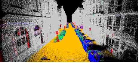
First, we test our framework on the Oakland 3D Point Cloud Dataset. Since the upper boundaryk = 100has been selected for reasons of computational costs, we have to take into account that it is likely to also represent 3D points which might favor a higher value. Accordingly, we consider the percentage of 3D points which are assigned neighborhoods withk < 100 neigh-bors which is98.12%and98.08%forNopt,dimandNopt,λ. For QDA-based classification based on all21features, the derived recall and precision values for different neighborhood definitions are provided in Table 2 and Table 3, and the respectiveF1-scores are visualized in Figure 3. The recall and precision values when using a RF classifier are provided in Table 4 and Table 5, and the respectiveF1-scores are visualized in Figure 4. For both clas-sifiers, it becomes visible that introducing an optimal neighbor-hood size for each individual 3D point has a beneficial impact on both recall and precision values, and consequently also on theF1 -score. Exemplary results for RF-based classification usingNopt,λ and all21features are illustrated in Figure 1 and Figure 5.
Oakland wire pole/trunk fac¸ade ground vegetation
N10 0.662 0.522 0.434 0.882 0.616
N50 0.667 0.507 0.473 0.916 0.788
N100 0.606 0.417 0.472 0.916 0.767
Nopt,dim 0.754 0.750 0.543 0.890 0.778
Nopt,λ 0.791 0.765 0.519 0.906 0.829
Table 2: Recall values for QDA-based classification using all fea-tures and different neighborhood definitions.
Oakland wire pole/trunk fac¸ade ground vegetation
N10 0.032 0.037 0.614 0.967 0.812
N50 0.035 0.079 0.832 0.977 0.805
N100 0.033 0.082 0.659 0.979 0.791
Nopt,dim 0.048 0.187 0.793 0.966 0.701
Nopt,λ 0.065 0.181 0.829 0.966 0.742
Table 3: Precision values for QDA-based classification using all features and different neighborhood definitions.
Oakland wire pole/trunk fac¸ade ground vegetation
N10 0.705 0.684 0.503 0.981 0.668
N50 0.578 0.617 0.679 0.988 0.779
N100 0.513 0.579 0.631 0.987 0.724
Nopt,dim 0.850 0.791 0.659 0.985 0.794
Nopt,λ 0.862 0.798 0.672 0.985 0.809
Table 4: Recall values for RF-based classification using all fea-tures and different neighborhood definitions.
If, besides the neighborhood definitions, the different feature sets are also taken into account, we get a total number of30possible combinations. For each combination, the resulting overall ac-curacy and mean class recall value are provided in Table 6 and
Oakland wire pole/trunk fac¸ade ground vegetation
N10 0.054 0.079 0.786 0.970 0.946
N50 0.048 0.196 0.845 0.979 0.942
N100 0.041 0.134 0.742 0.980 0.938
Nopt,dim 0.080 0.219 0.832 0.976 0.950
Nopt,λ 0.091 0.236 0.846 0.972 0.959
Table 5: Precision values for RF-based classification using all features and different neighborhood definitions.
wire
pole/trunk
fac¸ade ground vegetation
0
0.2
0.4
0.6
0.8
1
F
1
-score
N10 N50 N100
Nopt,dim
Nopt,λ
Figure 4:F1-scores for RF-based classification.
Figure 5: 3D point cloud with semantic labels assigned by the RF classifier (wire: blue, pole/trunk: red, fac¸ade: gray, ground: brown, vegetation: green).
Table 7 for QDA-based classification. The respective values for RF-based classification are provided in Table 8 and Table 9. Here, SCFS contains between12and14features, whereasSFCBF con-tains between6and8features. For both subsets, the respective features are distributed across all types of 3D and 2D features. The derived results clearly reveal that the feature subsetSdim is not sufficient for obtaining adequate classification results. In con-trast, using the feature subsetsS5,SCFSandSFCBFwhich are all based on feature relevance assessment yields classification results of better quality and, in particular when using a RF classifier, par-tially even a higher quality than the full feature setSall.
Oakland Sall Sdim Sλ,3D S5 SCFS SFCBF
N10 0.788 0.689 0.741 0.867 0.667 0.678
N50 0.850 0.771 0.822 0.927 0.725 0.762
N100 0.845 0.758 0.823 0.924 0.713 0.903
Nopt,dim 0.837 0.371 0.798 0.910 0.715 0.687
Nopt,λ 0.857 0.480 0.801 0.920 0.851 0.723
Table 6: Overall accuracy for QDA-based classification using dif-ferent neighborhood definitions and difdif-ferent feature sets.
Oakland Sall Sdim Sλ,3D S5 SCFS SFCBF
N10 0.623 0.365 0.454 0.583 0.570 0.618
N50 0.670 0.509 0.588 0.673 0.633 0.699
N100 0.636 0.474 0.555 0.668 0.600 0.708
Nopt,dim 0.743 0.440 0.561 0.666 0.694 0.703
Nopt,λ 0.762 0.477 0.576 0.704 0.755 0.739
Table 7: Mean class recall values for QDA-based classifica-tion using different neighborhood definiclassifica-tions and different feature sets.
Oakland Sall Sdim Sλ,3D S5 SCFS SFCBF
N10 0.875 0.579 0.742 0.887 0.873 0.857
N50 0.917 0.734 0.805 0.912 0.916 0.924
N100 0.901 0.728 0.814 0.901 0.902 0.920
Nopt,dim 0.918 0.696 0.773 0.915 0.918 0.907
Nopt,λ 0.922 0.628 0.851 0.911 0.924 0.923
Table 8: Overall accuracy for RF-based classification using dif-ferent neighborhood definitions and difdif-ferent feature sets.
Oakland Sall Sdim Sλ,3D S5 SCFS SFCBF
N10 0.708 0.483 0.598 0.686 0.699 0.702
N50 0.728 0.544 0.642 0.655 0.728 0.742
N100 0.687 0.504 0.612 0.638 0.693 0.697
Nopt,dim 0.816 0.615 0.676 0.754 0.812 0.808
Nopt,λ 0.825 0.596 0.692 0.759 0.827 0.825
Table 9: Mean class recall values for RF-based classification us-ing different neighborhood definitions and different feature sets.
recall and precision values using the feature setsSallandSCFSare provided in Table 10 as well as the resultingF1-scores. Based on the full feature setSall, the RF classifier provides an overall accu-racy of90.1%and a mean class recall of77.6%, whereas based on the feature subsetSCFS, a slight improvement to an overall accuracy of90.5%and a mean class recall of77.8%can be ob-served. A visualization for RF-based classification usingNopt,λ and all21features is provided in Figure 6.
Paris R P F1 R P F1
fac¸ade 0.957 0.962 0.960 0.958 0.964 0.961 ground 0.902 0.964 0.932 0.911 0.960 0.935 cars 0.606 0.755 0.672 0.603 0.768 0.676 motorcycles 0.639 0.123 0.206 0.657 0.136 0.225 traffic signs 0.974 0.055 0.105 0.978 0.058 0.109 pedestrians 0.575 0.019 0.036 0.559 0.020 0.038
Table 10: Recall (R), precision (P) andF1-score for RF-based classification involving all21features (left) and only the features inSCFS(right).
Figure 6: 3D point cloud with semantic labels assigned by the RF classifier (fac¸ade: gray, ground: brown, cars: blue, motorcycles: green, traffic signs: red, pedestrians: pink).
4 DISCUSSION
Certainly, a huge advantage of the proposed methodology is that it avoids the use of empiric or heuristic a priori knowledge on the scene with respect to neighborhood size. For the sake of gen-erality, involving such data-dependent knowledge should not be an option and the optimal neighborhood of each individual 3D point should be considered instead. This is in accordance with the idea that the optimal neighborhood size may not be the same for different classes and furthermore depend on the respective point density. In the provided Tables 2-5, the class-specific classifica-tion results clearly reveal that the suitability of all three neighbor-hood definitions based on a fixed scale parameter may vary from one class to the other. Instead, the approaches based on optimal neighborhood size selection address this issue and hence provide a significant improvement in recall and precision, and thus also in theF1-score over all classes (Figure 3 and Figure 4).
In particular, the detailed evaluation provides a clear evidence that the proposed approach for optimal neighborhood size selec-tion is beneficial in comparison to the other neighborhood defini-tions, since it often yields a significant improvement with respect to performance and behaves close to the best performance oth-erwise. A strong indicator for the quality of the derived results has been defined by the mean class recall, as only a high overall accuracy may not be sufficient for analyzing the derived results. For the Oakland 3D Point Cloud Dataset, for instance, we have an unbalanced test set and an overall accuracy of70.5%can be obtained if only the instances of the classground are correctly classified. This clear trend to overfitting becomes visible when considering the respective mean class recall of only20.0%.
In comparison to other recent investigations based on a fixed scale parameterk(Weinmann et al., 2013), the recall values are signif-icantly increased, and a slight improvement with respect to the precision values can be observed. Even in comparison to inves-tigations involving approaches of contextual learning (Munoz et al., 2009b), our methodology yields higher precision values with approximately the same recall values over all classes.
Considering the different feature sets (Tables 6-9), it becomes visible that the feature subsetSdim of the three dimensionality featuresLλ,PλandSλis not sufficient for 3D scene interpreta-tion. This might be due to ambiguities, since the classeswireand pole/trunkprovide a linear behavior, whereas the classesfac¸ade and ground provide a planar behavior. This can only be ade-quately handled by considering additional features. Even when only using the feature subsetSλ,3Dof the eigenvalue-based 3D features, the results are significantly worse than when using the full feature setSall. In contrast, the feature subsets derived via the three approaches for feature selection provide a performance close to the full feature setSallor even better. In particular, the feature subsetSCFSderived via Correlation-based Feature Selec-tion provides a good performance without being based on manu-ally selected parameters such as the feature subsetSFCBFderived via the Fast Correlation-Based Filter.
5 CONCLUSIONS AND FUTURE WORK
In this paper, we have addressed the interleaved issue of optimally describing 3D structures by geometrical features and selecting thebestfeatures among them as input for classification. We have presented a new, fully automatic and versatile framework for se-mantic 3D scene interpretation. The framework involves optimal neighborhood size selection which is based on minimizing the measure of eigenentropy over varying scales in order to derive optimized features with higher distinctiveness in the subsequent step of feature extraction. Further applying the measure of en-tropy for feature selection, irrelevant and redundant features are recognized based on a relatively small training set and, conse-quently, these features do not have to be calculated and stored for the test set. In a detailed evaluation, we have demonstrated the significant and beneficial impact of optimal neighborhood size selection, and that the selection of adequate feature subsets may even further increase the quality of 3D scene interpretation.
For future work, we plan to address the step from individual 3D point classification to a spatially smooth labeling of nearby 3D points. This could be based on probabilistic relaxation or smooth labeling techniques adapted from image processing.
ACKNOWLEDGEMENTS
REFERENCES
Belton, D. and Lichti, D. D., 2006. Classification and segmentation of ter-restrial laser scanner point clouds using local variance information.The International Archives of the Photogrammetry, Remote Sensing and Spa-tial Information Sciences, Vol. XXXVI, Part 5, pp. 44–49.
Breiman, L., 2001. Random forests.Machine Learning, 45(1), pp. 5–32.
Brodu, N. and Lague, D., 2012. 3D terrestrial lidar data classification of complex natural scenes using a multi-scale dimensionality criterion: applications in geomorphology. ISPRS Journal of Photogrammetry and Remote Sensing, 68, pp. 121–134.
Carlberg, M., Gao, P., Chen, G. and Zakhor, A., 2009. Classifying urban landscape in aerial lidar using 3D shape analysis. Proceedings of the IEEE International Conference on Image Processing, pp. 1701–1704.
Chehata, N., Guo, L. and Mallet, C., 2009. Airborne lidar feature se-lection for urban classification using random forests. The International Archives of the Photogrammetry, Remote Sensing and Spatial Informa-tion Sciences, Vol. XXXVIII, Part 3/W8, pp. 207–212.
Criminisi, A. and Shotton, J., 2013.Decision forests for computer vision and medical image analysis. Advances in Computer Vision and Pattern Recognition, Springer, London, UK.
Demantk´e, J., Mallet, C., David, N. and Vallet, B., 2011. Dimension-ality based scale selection in 3D lidar point clouds. The International Archives of the Photogrammetry, Remote Sensing and Spatial Informa-tion Sciences, Vol. XXXVIII, Part 5/W12, pp. 97–102.
Filin, S. and Pfeifer, N., 2005. Neighborhood systems for airborne laser data.Photogrammetric Engineering & Remote Sensing, 71(6), pp. 743– 755.
Goulette, F., Nashashibi, F., Abuhadrous, I., Ammoun, S. and Laurgeau, C., 2006. An integrated on-board laser range sensing system for on-the-way city and road modelling. The International Archives of the Pho-togrammetry, Remote Sensing and Spatial Information Sciences, Vol. XXXVI, Part 1.
Guyon, I. and Elisseeff, A., 2003. An introduction to variable and feature selection.Journal of Machine Learning Research, 3, pp. 1157–1182.
Hall, M. A., 1999. Correlation-based feature subset selection for machine learning. PhD thesis, Department of Computer Science, University of Waikato, New Zealand.
Hu, H., Munoz, D., Bagnell, J. A. and Hebert, M., 2013. Efficient 3-D scene analysis from streaming data. Proceedings of the IEEE Interna-tional Conference on Robotics and Automation, pp. 2297–2304.
Khoshelham, K. and Oude Elberink, S. J., 2012. Role of dimensionality reduction in segment-based classification of damaged building roofs in airborne laser scanning data.Proceedings of the International Conference on Geographic Object Based Image Analysis, pp. 372–377.
Lafarge, F. and Mallet, C., 2012. Creating large-scale city models from 3D-point clouds: a robust approach with hybrid representation. Interna-tional Journal of Computer Vision, 99(1), pp. 69–85.
Lalonde, J.-F., Unnikrishnan, R., Vandapel, N. and Hebert, M., 2005. Scale selection for classification of point-sampled 3D surfaces. Proceed-ings of the International Conference on 3-D Digital Imaging and Model-ing, pp. 285–292.
Lee, I. and Schenk, T., 2002. Perceptual organization of 3D surface points.The International Archives of the Photogrammetry, Remote Sens-ing and Spatial Information Sciences, Vol. XXXIV, Part 3A, pp. 193–198.
Linsen, L. and Prautzsch, H., 2001. Natural terrain classification using three-dimensional ladar data for ground robot mobility. Proceedings of Eurographics, pp. 257–263.
Liu, H., Motoda, H., Setiono, R. and Zhao, Z., 2010. Feature selection: an ever evolving frontier in data mining.Proceedings of the Fourth Inter-national Workshop on Feature Selection in Data Mining, pp. 4–13.
Lodha, S. K., Fitzpatrick, D. M. and Helmbold, D. P., 2007. Aerial li-dar data classification using AdaBoost.Proceedings of the International Conference on 3-D Digital Imaging and Modeling, pp. 435–442.
Mallet, C., Bretar, F., Roux, M., Soergel, U. and Heipke, C., 2011. Rele-vance assessment of full-waveform lidar data for urban area classification. ISPRS Journal of Photogrammetry and Remote Sensing, 66(6), pp. S71– S84.
Mitra, N. J. and Nguyen, A., 2003. Estimating surface normals in noisy point cloud data. Proceedings of the Annual Symposium on Computa-tional Geometry, pp. 322–328.
Munoz, D., Bagnell, J. A., Vandapel, N. and Hebert, M., 2009a. Con-textual classification with functional max-margin Markov networks. Pro-ceedings of the IEEE Conference on Computer Vision and Pattern Recog-nition, pp. 975–982.
Munoz, D., Vandapel, N. and Hebert, M., 2009b. Onboard contextual classification of 3-D point clouds with learned high-order Markov random fields.Proceedings of the IEEE International Conference on Robotics and Automation, pp. 2009–2016.
Niemeyer, J., Rottensteiner, F. and Soergel, U., 2012. Conditional random fields for lidar point cloud classification in complex urban areas. ISPRS Annals of the Photogrammetry, Remote Sensing and Spatial Information Sciences, Vol. I-3, pp. 263–268.
Niemeyer, J., Rottensteiner, F. and Soergel, U., 2014. Contextual classi-fication of lidar data and building object detection in urban areas.ISPRS Journal of Photogrammetry and Remote Sensing, 87, pp. 152–165. Pauly, M., Keiser, R. and Gross, M., 2003. Multi-scale feature extraction on point-sampled surfaces.Computer Graphics Forum, 22(3), pp. 81–89. Press, W. H., Flannery, B. P., Teukolsky, S. A. and Vetterling, W. T., 1988. Numerical recipes in C. Cambridge University Press, Cambridge, UK. Pu, S., Rutzinger, M., Vosselman, G. and Oude Elberink, S., 2011. Recog-nizing basic structures from mobile laser scanning data for road inventory studies. ISPRS Journal of Photogrammetry and Remote Sensing, 66(6), pp. S28–S39.
Quinlan, J. R., 1986. Induction of decision trees.Machine Learning, 1(1), pp. 81–106.
Schindler, K., 2012. An overview and comparison of smooth labeling methods for land-cover classification.IEEE Transactions on Geoscience and Remote Sensing, 50(11), pp. 4534–4545.
Secord, J. and Zakhor, A., 2007. Tree detection in urban regions using aerial lidar and image data. IEEE Geoscience and Remote Sensing Let-ters, 4(2), pp. 196–200.
Serna, A. and Marcotegui, B., 2013. Urban accessibility diagnosis from mobile laser scanning data. ISPRS Journal of Photogrammetry and Re-mote Sensing, 84, pp. 23–32.
Serna, A., Marcotegui, B., Goulette, F. and Deschaud, J.-E., 2014. Paris-rue-Madame database: a 3D mobile laser scanner dataset for benchmark-ing urban detection, segmentation and classification methods. Proceed-ings of the International Conference on Pattern Recognition Applications and Methods, pp. 819–824.
Shannon, C. E., 1948. A mathematical theory of communication. The Bell System Technical Journal, 27(3), pp. 379–423.
Shapovalov, R., Velizhev, A. and Barinova, O., 2010. Non-associative Markov networks for 3D point cloud classification. The International Archives of the Photogrammetry, Remote Sensing and Spatial Information Sciences, Vol. XXXVIII, Part 3A, pp. 103–108.
Shapovalov, R., Vetrov, D. and Kohli, P., 2013. Spatial inference ma-chines. Proceedings of the IEEE Conference on Computer Vision and Pattern Recognition, pp. 2985–2992.
Tokarczyk, P., Wegner, J. D., Walk, S. and Schindler, K., 2013. Beyond hand-crafted features in remote sensing.ISPRS Annals of the Photogram-metry, Remote Sensing and Spatial Information Sciences, Vol. II-3/W1, pp. 35–40.
Velizhev, A., Shapovalov, R. and Schindler, K., 2012. Implicit shape models for object detection in 3D point clouds. ISPRS Annals of the Photogrammetry, Remote Sensing and Spatial Information Sciences, Vol. I-3, pp. 179–184.
Weinmann, M., Jutzi, B. and Mallet, C., 2013. Feature relevance as-sessment for the semantic interpretation of 3D point cloud data. ISPRS Annals of the Photogrammetry, Remote Sensing and Spatial Information Sciences, Vol. II-5/W2, pp. 313–318.
Xiong, X., Munoz, D., Bagnell, J. A. and Hebert, M., 2011. 3-D scene analysis via sequenced predictions over points and regions. Proceed-ings of the IEEE International Conference on Robotics and Automation, pp. 2609–2616.
Xu, S., Vosselman, G. and Oude Elberink, S., 2014. Multiple-entity based classification of airborne laser scanning data in urban areas.ISPRS Jour-nal of Photogrammetry and Remote Sensing, 88, pp. 1–15.
Yu, L. and Liu, H., 2003. Feature selection for high-dimensional data: a fast correlation-based filter solution. Proceedings of the International Conference on Machine Learning, pp. 856–863.