Modeling plume behavior for nonlinearly
sorbing solutes in saturated homogeneous
porous media
A. Abulaban
a ,*, J. L. Nieber
b& D. Misra
c aDepartment of Biosystems and Agricultural Engineering, University of Minnesota, St Paul, MN, USA b
Department of Biosystems and Agricultural Engineering, University of Minnesota, St Paul, MN, USA c
Army High Performance Computing Research Center, University of Minnesota, Minneapolis, MN, USA
(Received 15 March 1996; revised 8 January 1997; accepted 29 January 1997)
Transport of a sorbing solute in a two-dimensional steady and uniform flow field is modeled using a particle tracking random walk method. The solute is initially introduced from an instantaneous point source. Cases of linear and nonlinear sorption isotherms are considered. Local pore velocity and mechanical dispersion are used to describe the solute transport mechanisms at the local scale. The numerical simulation of solute particle transport yields the large scale behavior of the solute plume. Behavior of the plume is quantified in terms of the center-of-mass displacement distance, relative velocity of the center-of-mass, mass breakthrough curves, spread variance, and longitudinal skewness. The nonlinear sorption isotherm affects the plume behavior in the following way relative to the linear isotherm: (1) the plume velocity decreases exponentially with time; (2) the longitudinal variance increases nonlinearly with time; (3) the solute front is steepened and tailing is enhanced.q1998 Elsevier Science Limited. All rights reserved.
Key words: solute transport, Freundlich nonlinear sorption, saturated flow, particle tracking-random walk, retardation.
1 INTRODUCTION
Sorption is probably the major factor controlling the move-ment of many hazardous substances through the vadose zone and in ground water aquifers.49 The term sorption refers to the physical/chemical attachment (adsorption) and detachment (desorption) of some chemical to a solid surface such as a porous medium solid. The system strives to attain equilibrium between adsorbed and desorbed phases. Equilibrium times vary for different chemicals and porous media types. However, for most chemicals of con-cern in ground water and different porous media types, equilibrium times are of the order of minutes to hours. Equilibrium times have been reported for an extensive list of chemicals in different soil environments to have a maximum of 72 h, and to be less than 24 h for most common chemicals.15 In the context of groundwater flow
and transport these equilibrium times are considerably small. Therefore, the Local Equilibrium Assumption (LEA) seems to be a reasonable approximation to adopt in most instances.
A primary issue of solute transport is the definition of an appropriate value for dispersivity. The assignment of laboratory-scale dispersivities to field scale problems has been found to underestimate plume spreading compared to field observed behavior.31,45,46 One way to circumvent this problem is to scale up the laboratory-scale dispersion coefficients,33 but this generally results in overestimation of dispersion close to the source.32 The problem of defining a unique dispersivity relates to the fact that the dispersivity commonly increases with distance travelled as the transported mass encounters successively larger scales of heterogeneity.14
To better represent the scale dependence of dispersivity it is necessary to account for variability at the smallest scale possible. In porous media, mixing at the junctions of the Advances in Water Resources 21 (1998) 487–498
q1998 Elsevier Science Limited All rights reserved. Printed in Great Britain 0309-1708/98/$19.00 + 0.00
PII: S 0 3 0 9 - 1 7 0 8 ( 9 7 ) 0 0 0 0 7 - 9
487
flow paths at the pore scale is the major cause of hydro-dynamic dispersion.10However, modeling at the pore-scale is prohibitive when applying the model to large scale effects. Hence, the minimum scale possible is the Darcy-scale or continuum Darcy-scale,6 where pore–scale effects are represented by core-scale measured dispersivities. With spatial discretizations given at the core-scale it is possible to represent the scale-dependent dispersivity with appro-priate computational models for solute transport.
In this paper we utilize the particle tracking random walk (PTRW) method3,17,47 to examine the behavior of solute plumes initiated from an instantaneous point source in a uniform flow field. We examine cases of solutes which obey linear and Freundlich sorption isotherms. The results presented are a lead into the evaluation of plume behavior in hydraulically and chemically heterogeneous domains. Related studies have been reported by Tompson40 and Bosma and van der Zee,8 who considered only a single Freundlich isotherm and emphasized only the first two spatial moments of the solute plume. More recently, Bosma et al.9 considered several Freundlich isotherms, but used Monte Carlo simulations to predict average plume behavior in terms of the first two spatial moments. In this paper we show the sensitivity of plume behavior to the Freundlich isotherm exponent, in terms of spatial moments, including plume skewness, as well as mass break-through curves. Also we look at the dilution of the peak concentration, as well as the total solute mass in liquid phase which varies due to nonlinearity in the Freundlich isotherm.
2 THE TRANSPORT MODEL
The transport of a sorbing chemical can be described by the advection–dispersion–sorption equation:
where C is the concentration in the liquid phase (ML¹3); S is the concentration in the adsorbed phase expressed as mass of solute per mass of solid (1); v is the local velocity vector (LT¹1); D is the local hydrodynamic dispersion tensor10 (LT¹2); r is the dry bulk density of the porous matrix (ML¹3);Fis the effective porosity (1); and t is the time variable (T).
The hydrodynamic dispersion tensor can be written as,5,6,30
D¼(aTVþDm)Iþ(aL¹aT)
vv
V (2)
where Dmis the molecular diffusion coefficient (L2T
¹1); I
is the identity matrix; V is the magnitude of the velocity vector (LT¹1);aLandaTare, respectively, the longitudinal and transverse dispersivities (L); and vv is the diadic of the velocity vector. Utilizing the identity
=2:(DC)¼=·(D·=C)¹(=C)·(=·D)
where=·Dis a velocity-like term that prevents the accumu-lation of solute in stagnation zones.37,38
Rearranging terms, eqn (3) can be written as
] dependent retardation coefficient, R(C,x). The expression inside the time derivative is the total (sorbed plus dis-solved) solute concentration, CT ¼ R(C,x)C. Substituting
C¼CT=R(C,x) in eqn (4) results in the transport equation in terms of the total solute concentration, CT:
]CT
D=R(C,x) are the retarded velocity and dispersion tensor,
respectively.
Several mechanistic and phenomenological relation-ships have been derived to describe the equilibrium concen-trations in the solid and fluid phases.48The most commonly used among those relationships is the Freundlich iso-therm,13,15,28,35,48expressed as
S¼Kfð ÞxC n
(6)
where Kf(x)((L3M¹1)n) relates to sorption capacity, while n relates to sorption intensity. Using the Freundlich isotherm to express S in terms of C the retardation coefficient can be written as
R(C,x)¼1þa xð ÞCn¹1 (7)
where a xð Þ ¼(rð ÞxKfð Þ)x =Fð Þ.x
Although the linear version (n¼1.0) of the Freundlich isotherm has been widely used to model the transport of sorbing chemicals,11,23,26it has become increasingly appar-ent that this model frequappar-ently fails to provide adequate representation of the effects of sorption processes on con-taminant transport.48 Nonlinear isotherms often represent equilibrium sorption phenomena more satisfactorily. Even for slight nonlinearity in the isotherm Weber et al.48showed that plume behavior, in terms of center-of-mass retardation, tailing of breakthrough, and front sharpening, was drasti-cally affected for an isotherm exponent of 0.95 in contrast with that for a linear isotherm. Tailing of breakthrough curves is commonly perceived to be a result of kinetic pro-cesses,43while in the case of a nonlinear isotherm it occurs because solute retardation increases exponentially as the concentration decreases.
hysteresis.27Such a non-unique relationship, however, will make the simulation process more complicated, similar to the increased complexities involved in modeling unsatu-rated flow processes with hysteresis in the water retention function.24
It should be apparent from eqn (5) that the retardation coefficient is a critical factor in the transport equation and in the development of the solute plume. Therefore, it would be of help to shed some light on its behavior.
As can be seen from eqn (7) above, the retardation coeffi-cient for the case of a linear isotherm is
R(x)¼1þrð Þx Kdð Þx
Fð Þx (8)
which is dependent on the spatially-variable sorption capa-city coefficient, dry bulk density, and porosity. In this case the transport equation is the linear PDE for a nonreactive solute scaled by the retardation coefficient. The parameter
Kd(x) above is the special case of the sorption capacity for the linear isotherm, and is commonly known as the distri-bution (or partition) coefficient.
For nonlinear isotherms it can be readily seen from eqn (7) that: (1) the retardation coefficient is proportional to the sorption capacity; (2) the retardation coefficient increases nonlinearly with decreasing concentration; and (3) the effect of the isotherm exponent on the retardation coefficient depends on the concentration magnitude.
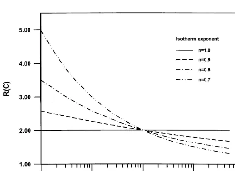
For the range of values of n used in this paper (0.7#n# 1.0), Fig. 1 illustrates the behavior of the retardation coeffi-cient for a wide range of concentrations for the special case when a(x)¼1.0, that is R(C,x)¼1þCn¹1¼RðCÞ. Exam-ination of Fig. 1 shows that for concentrations greater than 1.0 mg/l, R(C) increases with the Freundlich isotherm n. For concentrations below 1.0 mg/l the trend is reversed; R(C) decreases as n increases. Also the values of R(C) in this case are much larger than in the case of large concentrations. Note that when n¼1.0, Cn¹1¼1.0, and therefore R(C) is constant and is equal to 1þa(x).
Due to hydrodynamic dispersion, concentrations within
the plume decrease towards the edges of the plume. For any exponent less than 1.0, the retarded velocities on the edges of the plume will be smaller than the velocity of the peak, and hence the solute closer to the peak of the plume will be moving faster than that at the edges. Thus as local dispersion tends to spread the plume and dilute the concentration, the retardation coefficient increases across the advancing front of the plume and slows its progress. This can be construed as a self-restraining process imposed by the plume itself, that is, the plume tends to resist hydrodynamic dispersion. This produces a sharpening front, because the solute within the plume moves faster than the advancing front. On the other hand, as the solute leaves sites along the trailing edge of the plume the retardation coefficient increases and hence hinders solute removal. As concentration approaches zero, the retardation coefficient tends to infinity, meaning that at very small concentrations solute will hardly be moving. The result will, therefore, be an ever stretching tail of the plume. Theoretically the tail of the plume should extend back at least to the injection point (it may travel a short distance along the upgradient of the injection point due to local dis-persion). The implication of the Freundlich isotherm is that, in theory, since the retardation coefficient tends to infinity as concentration vanishes, once solute invades a site it will never be totally recovered.
3 SOLUTION PROCEDURE
When used to solve the advection–dispersion–sorption equation, conventional computational techniques, such as finite difference and finite element methods, suffer from numerical complications chief among which is numerical dispersion. The numerical dispersion results when there are sudden spatial and temporal changes of solute concen-trations. Operator splitting methods are one means to improve the solution accuracy.16,25However, the computa-tional costs involved with any of these techniques is gener-ally high, inhibiting applications of these methods to large flow domains.
An alternative to the conventional numerical techniques for solute transport is the particle tracking-random walk (PTRW) method where a solute plume is represented with a large number of particles that move according to spatially and/or temporally variable local velocities (deterministic translation). A random component proportional to the local dispersivity of the porous medium is added to the deterministic translation of a particle to account for the Brownian-like motion caused by heterogeneities at scales smaller than the Darcy scale.
The use of the PTRW technique to model transport of solutes with dispersion has been shown to be superior in accuracy, efficiency, and computational cost compared to more conventional finite difference and finite element schemes.19–21,37,38In addition to its application for model-ing solute transport in porous media,3,17,21,33,34,37,38,41,42,47 the PTRW technique has been applied to transport problems Fig. 1. Behavior of the retardation coefficient function for the case
in free water bodies, where random motions are the result of turbulence in flow velocities. PTRW techniques have also been used successfully for the simulation of dispersion in turbulent boundary layers,4 effluent plumes,7,18 effluent patches,2,18and in the ocean.19
Like other numerical methods that approximate continu-ous variables with discretized ones, the PTRW method also suffers some drawbacks. One such drawback is the wide oscillations that occur at locations when numbers of parti-cles are too small, which can occur at the leading and trail-ing edges of a solute plume. This problem can be improved by increasing the number of particles or by using a concentra-tion smoothing technique.39Another way to improve the solu-tion is by increasing particle resolusolu-tion at low-concentrasolu-tion sites. In the present application we used 200 000 particles, which we found to be large enough to minimize concentra-tion oscillaconcentra-tions during the simulaconcentra-tion times considered.
The mathematical foundation for the PTRW technique lies in the similarity between the advection/dispersion trans-port equation6 and the Fokker–Planck equation,12,29,36 a conservation equation for the probability distribution of particles moving independently in a random field. Detailed mathematical development of the PTRW technique and its application to simulate contaminant transport in porous media can be found in Tompson et al.37and Abulaban.1
The motion of a particle moving in a random field can be described by the nonlinear Langevin equation12
dX
dt ¼A X(t),t
ÿ
þBÿX(t),t
·yð Þt (9)
where X(t) is the position of the particle at time t. The vector A(X,t) is a known function of space and time, and is used to represent the deterministic driving forces acting to change X. The second order tensor B(X,t) is also a
known function of space and time that aligns the random forces with A(X,t). The vectory(t) represents the uncorre-lated and rapidly changing random forces. Integration of the Langevin equation over a smallDt yields the discretized
stepping equation
DX¼A Xÿ (t),tDtþBÿX(t),t·yð ÞDt t (10)
If a large number of independently moving particles started from the initial position X0 at t0, then the fraction
of particles expected to be found in a small volume around the point X at time t, denoted f(X,t/X0,t0), will obey the
Fokker–Planck conservation equation12,29,44given by
]f
Comparing the Fokker–Planck equation, eqn (11), with the transport equation, eqn (5), we can see that if vr and
Drare not dependent on CT(through C), as is the case for conservative and for linearly sorbing solutes, then the solute transport equation and the Fokker–Planck equation will be equivalent if A andBare chosen such that
A¼vr; BB T
¼2Dr (12)
while f corresponds to CT. However, vr and Dr for non-linearly sorbing solutes are concentration-dependent, which means that the particles will not move independently; the movement of a particle depends on the intensity of particles around it. This is a violation of the assumption of indepen-dence used to derive the Fokker–Planck equation. Thus it is necessary to adjust for this dependence in the application of the method. The issue of particle dependence has not been addressed explicitly in any of the previous applications8,9,40 of the analogy to the solution of transport with nonlinear sorption.
The problem of particle movement dependence can be circumvented by an iterative solution procedure.22 The way in which the iterative procedure circumvents the dependence of particles can be explained by using an argu-ment based on the existence of an analytical solution. Let us suppose that an analytical solution to the nonlinear sorp-tion problem is known. Then the retardasorp-tion coefficient distribution will be known exactly for all time and all space. If one were to then use this distribution in moving a set of particles, the particles can be moved independently because the retardation coefficients do not depend on parti-cle movement, but instead are known a priori. The applica-tion of the Fokker–Planck analogy for such a condiapplica-tion is exact.
With the iterative solution, the appropriate spatial distri-bution of the retardation coefficient for a particular time step is determined by repeated trial (iterative) movements of the particles until a specified convergence criterion is satisfied. Note that within any particular iteration, a trial retardation coefficient distribution is used and the particles are assumed to move independently of each other. Thus, for each iteration, the application of the Fokker–Planck analogy is exact. The distribution of the particles at the end of the time step following such an iterative procedure will be the same as the distribution that would be computed with independently moving particles using the retardation coefficient distribution had it been known a priori. We can therefore conclude that the application of the Fokker– Planck analogy to the case of nonlinear sorption is valid when iteration is used to account for dependence among particle movements.
In our application of iteration the retardation field for a new time step is initiated using the current retardation field. The particles are then moved and a retardation coefficient field is calculated for the final positions of the particles. The retardation coefficient field is then averaged between that for the initial field and the final field. The particles are moved again, starting from their positions at the beginning of the time step. Iterations continue until the retardation field does not change appreciably.
retarded velocity and dispersion, but with a different random component since each particle uses a different ran-dom number. It should be noted here that, in order to avoid random changes in the retardation coefficient field due to random numbers, in our application a set of random num-bers is generated at the beginning of each time step and the set is used for all the iterations within that time step. We found that the retardation coefficient field generally converged within three or four iterations.
Experience with the numerical solution showed that errors due to not iterating the solution depend on initial conditions, number of particles used to represent the total solute mass, length of the solution time step, as well as the nonlinearity of the sorption isotherm. The error increased for higher initial concentrations, smaller injection area, lar-ger time steps, and stronlar-ger nonlinearity in the sorption isotherm. Also errors grow with time into the simulation. The quantitative effect of not iterating on the retardation coefficient has not been reported in the literature.
Other computational aspects related to the implementa-tion of the random walk technique for conservative solutes are discussed in detail by Tompson et al.37and Tompson.40 Inserting A andBback into eqn (10) yields the stepping
equation
Xm¼Xm¹1þvrDtmþB·wm (13)
where the subscript m indicates the time level,Dtm¼tm¹
tm¹1, and wm contains the random component. In the present application the flow field is homogeneous and therefore the divergence of the dispersion tensor within the vrterm vanishes.
By the central limit theorem the random component wm can take any form, provided that it possesses a zero-mean and a variance proportional toDtm. Therefore, it will suffice to use a standardized random vector, Z, whose components
Zi (i ¼ x,y,z) are statistically independent with a zero-mean and a unit variance such that wm¼Z
Dtm
p
. Conse-quently, any of a wide range of distributions can be imple-mented, such as a normal N(0,1) distribution,3or a simple uniform distribution spread over 6Î3 to represent the Zi components.
4 RESULTS
Whereas it is recognized that the hydraulic properties as well as chemical properties are usually spatially variable in a flow field, results are presented in this paper for a physically and chemically homogeneous flow field. This paper is intended as background for a subsequent paper to consider spatial heterogeneity of the hydraulic conductivity and the sorption capacity.
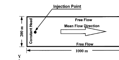
The flow field illustrated in Fig. 2 is a 1000 m by 200 m rectangle with one-dimensional flow along the longer dimension of the domain. Parameters are assumed to be constant with depth, so a 1.0 m slice is considered. The dimensions were chosen to be large enough to allow us to
observe the behavior of the plume at large times where the concentrations become very small. Since this is a nonlinear problem, large scale behavior cannot be deduced from Monte Carlo simulations similar to those of Bosma and van der Zee8and Bosma et al.9The boundaries are treated as absorbing boundaries where the solute particles are allowed to cross the boundaries and leave the flow domain forever. This treatment is similar to that of Tompson and Gelhar38and Bosma et al.,9whereas Schwartz31and Smith and Schwartz33,34 treated the boundaries as reflecting boundaries.
The flow domain was discretized into 1-m square cells. Solute is injected as an instantaneous pulse in the horizontal plane. To avoid very high initial concentrations the solute is uniformly distributed over a square region containing 16 cells centered in the middle of the transverse direction and 10 m downgradient from the inflow boundary of the domain to ensure that no solute would cross the inflow boundary early in the simulation.
The mean flow velocity was 1.0 m/day in the x-direction. The effective porosity was constant at 0.35, and the soil bulk density was 1.75 g/cm3. Longitudinal and transverse disper-sivities were 0.5 m and 0.1 m, respectively. The sorption capacity factor for all isotherms was 0.2 (1/g)n, which was chosen to give a retardation coefficient of 2.0 for the linear case. Four simulations were performed using 200 g of solute and varying the isotherm exponents over four values: 0.7, 0.8, 0.9, and 1.0. The initial liquid concentration depends on the value of the exponent, n. Initial liquid concentrations for the different exponent values used are summarized in Table 1. The number of particles used to represent the solute was 200 000 with a constant particle mass, mp, of 1.0 mg. The particles carry the total mass and move with the local retarded velocities. Even though only the dissolved mass is available to move with the flow velocity, the instantaneous equilibrium assumption makes it appear like all the mass is moving with a phase-averaged velocity which can be easily shown to be the flow velocity divided by the retardation coefficient.
Results are presented below in terms of concentration profiles, mass breakthrough, plume velocity, spread vari-ance, and plume skewness. For all of the simulations the plumes are symmetric in the transverse direction due to the one-dimensional flow, and, except for the spread Fig. 2. Size and orientation of the flow domain. Also shown are the boundary conditions, mean velocity direction, and location of
variance, the transverse moments were unremarkable. Results were, therefore, evaluated in terms of the longi-tudinal spatial moments and breakthrough curves, as well as the transverse spread variance. Mathematical definitions of the spatial moments can be found elsewhere.1,38In our simulations moments are estimated from cell concentrations assigned to the centers of the cells as:
X1(t)¼
F
M(t)
XNc
j¼1
xjCj(t)DxDy (14)
X112(t)¼
F
M(t)
XNc
j¼1
(xj¹X1(t)) 2
Cj(t)DxDy (15)
X222(t)¼
F
M(t)
XNc
j¼1
(yj¹X2(t)) 2
Cj(t)DxDy (16)
ˆ
Cs,1¼
1 (X11)3
=2
F
M(t)
XNc
j¼1
(xj¹X1(t))3Cj(t)DxDy
" #
(17)
where M(t) is the total mass in liquid, calculated as:
M(t)¼FX Nc
j¼1
CjDxDy (18)
In the expressions above Cj is the concentration in the computational cell, Nc is the number of computational cells in the domain, and Dx and Dy are the lengths of
the rectangular computational cells in the longitudinal and transverse directions, respectively, and xj and yj are the coordinates of the center of computational cell j. Also
X1is the longitudinal position of the center of mass, X112 and X22
2
are the longitudinal and transverse spread variances about the center of mass, respectively, and Cˆs,1is the long-itudinal coefficient of skewness. Note that the longlong-itudinal displacement is X1(t)¹X1(0).
The cell liquid concentration, Cj, is calculated by solving the balance equation relating the total mass in a cell with the dissolved phase concentration. The total mass in a cell, Mj, is the sum of the masses of all the particles in that cell, Njmp, where Njis the number of particles in the cell. This total mass is distributed between the dissolved phase, Cj, and adsorbed phase, Sj ¼ KfCjn, according to the following
balance equation:
DxDy(FCjþrC n
j)¼Mj (19)
For a linear isotherm (n¼1.0) eqn (19) is linear and there-fore it is solved directly to give Cjas the total mass divided by the retardation coefficient given by eqn (8). For non-linear isotherms, however, eqn (19) is nonnon-linear and is solved numerically using the Newton–Raphson method.
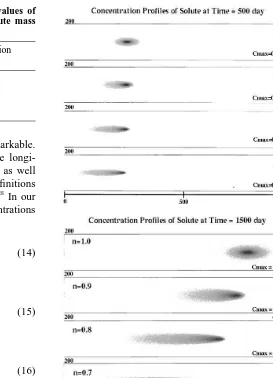
An example of the concentration distribution in the plumes for the various isotherm exponents is presented in Fig. 3. The plumes are illustrated for 500 and 1500 days. It is seen that the plume is virtually symmetric for the linear isotherm case, which is the expected behavior since the transport equation is linear and the Peclet number is 2.0. In contrast, the plumes for the nonlinear cases have sharp fronts and long tails, and the tails increase in length as the isotherm exponent decreases.
As has been discussed earlier the tail should extend back to the injection point, but this does not appear to be the case (Fig. 3). The reason is that there is a minimum concentration that can be resolved in each case due to numerical limita-tions. The smallest resolvable concentration and the largest Table 1. Initial liquid concentrations for different values of
isotherm exponent corresponding to an injected solute mass of 200 g
Isotherm exponent Initial liquid concentration (mg/l)
1.0 17.85
0.9 21.49
0.8 25.16
0.7 28.42
corresponding retardation coefficient depend on the value of the Freundlich exponent. They correspond to the concentra-tion resulting from one particle in a computaconcentra-tional cell. With 200 000 particles carrying 200 g of solute the smallest concentrations and the corresponding retardation coeffi-cients are given in Table 2.
The plume velocity is defined as the instantaneous time-derivative of the plume center of mass. The plume retardation coefficient can be defined as the inverse of the ratio of the plume velocity to the flow velocity.40Fig. 4 shows such a retardation coefficient for the different isotherm exponents. It is readily seen in this figure that the plume velocity remains constant for the linear isotherm, which is due to the fact that the retardation coefficient does not depend on concentration. In contrast, the plume velocities for all the nonlinear iso-therms decrease with time due to the global decrease in concentration. It is observed that initially the plume for n¼ 0.7 is the fastest, and the speed decreases with increasing n. Shortly after that the plume for the linear isotherm becomes the fastest and the velocity decreases with decreasing n. Table 2. Smallest resolvable solute concentrations and the cor-responding retardation coefficients when using 200 000 parti-cles to represent a mass of 200 g of chemical, for various values of the Freundlich isotherm exponent
Freundlich exponent
Smallest concentration (mg/l)
Retardation coefficient
1.0 0.0143 2.00
0.9 0.0111 2.57
0.8 0.0078 3.64
0.7 0.0047 6.00
Fig. 4. Longitudinal velocity of the plume center of mass.
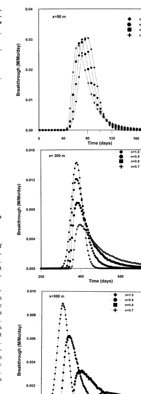
Fig. 5. Breakthrough curves at three cross-sections located at (a) 50 m, (b) 200 m, and (c) 500 m downgradient from the inflow
A theoretical assessment requires that the displace-ment for each of the nonlinear isotherms be asymptotic to some constant value at large time. This is due to the increasing retardation as the concentration decreases. As the concentration approaches zero, the retarded velocity also approaches zero, and the plume will then become stag-nant. In their analysis of large time behavior, Bosma et al.9 derived a relationship for the center of mass displacement. Differentiating their equation with respect to time gives the plume velocity, which tends to zero as t→`.
The longitudinal breakthrough curves at the cross-sections 50 m, 200 m, and 500 m are shown in Fig. 5 in terms of the rate of mass that crossed a cross-section within a time step. The curves were slightly smoothed by taking the 7-point moving average of the relative mass flux across the corresponding cross-section. As expected, the curves for the linear isotherm are symmetric. The curves for the nonlinear isotherms, however, show the sharpening fronts and the elongating tails of the plume. The slowing speed of the plume is also clear in Fig. 5 where we see that at the 50 m cross-section the curve for the n¼0.7 exponent appears first and the one for n¼1.0 comes last, while for the 200 m and 500 m cross-sections the curve for n¼1.0 comes first and the one for n¼0.7 comes last. The behavior of the breakthrough curves also indicates that the plumes for the nonlinear isotherms are skewed to the left, which is due to the sharp fronts and long tails.
The longitudinal spread variance of the plume for the different values of the Freundlich exponent used is shown in Fig. 6. It is obvious that the variance increases rapidly for smaller values of the exponent. It can also be seen that, except for the linear isotherm case (n ¼ 1.0) where the time dependence is linear, the variance grows in a nonlinear fashion. The nonlinearity of the growth is shown to be stronger for smaller n values. As was discussed previously,
the solute plume should slow asymptotically to zero due to increasing retardation with decreasing concentration, and thus we should expect the plume variance for the nonlinear cases to level off. This argument is supported by the theoretical large time behavior of the longitudinal spread variance as expressed by eqn (28) of Bosma et
al.9The time derivative of this equation tends to zero as
t → `.
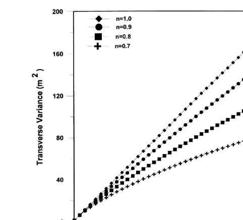
The transverse spread variance is shown in Fig. 7. Con-trary to the behavior of the longitudinal variance, Fig. 7 shows the transverse spread variance to decrease as the isotherm exponent decreases. This means that spreading is hindered in the direction of zero velocity. In fact, as was discussed earlier, the large longitudinal variances are largely due to the elongating tails, and the same behavior responsible for sharpening the leading front also causes the slower transverse spreading.
Because the ratio between the solute mass in the liquid phase and that in the adsorbed phase decreases as concen-tration decreases for the nonlinear cases, the total mass in the liquid phase decreases as the plume spreads. Illustrated in Fig. 8(a) is the ratio of total solute mass in liquid phase to the total injected mass. This is the inverse of another plume retardation defined as the total solute mass divided by the total mass in the liquid phase.40It is obvious from Fig. 8(a) that the liquid mass for the linear isotherm remains constant, which is due to the retardation coefficient being independent of concentration. However, the behavior for the nonlinear isotherms indicates that the plume retardation as defined above increases, a behavior similar to that of the retardation coefficient defined with the velocity of the plume center of mass relative to the flow velocity and depicted in Fig. 4. The relationships depicted in Fig. 8(a) are important for clean-up efforts. Since we know that for the nonlinear cases the more spread the solute is, the more Fig. 6. Longitudinal spread variance of the solute plume.
strongly it adsorbs to the solid, clean-up will be significantly enhanced by doing it earlier.
Another behavior related to the spreading of the plume is that of the peak concentration. Shown in Fig. 8(b) is the peak concentration normalized by the initial peak concen-tration. It should be noted here that since the total injected solute mass is the same for the different isotherm exponents, and because of the different partitioning behavior with the different isotherm exponents, the initial peak concentrations are different. In fact Fig. 8(a) shows that initially the total mass in the liquid phase, and thus the initial concentration, are largest for the smallest isotherm exponent and they decrease as the exponent increases. It is interesting to see from Fig. 8(b) that the normalized peak concentration does
not change appreciably with the isotherm exponent, espe-cially after we saw the great increase of the longitudinal spread variance with decreasing the isotherm exponent. This is further evidence that the enhancement of the long-itudinal spread variance is due to the elongating tail, and that spreading in the nonlinear cases is actually increased stretching of the tail rather than dilution of the peak.
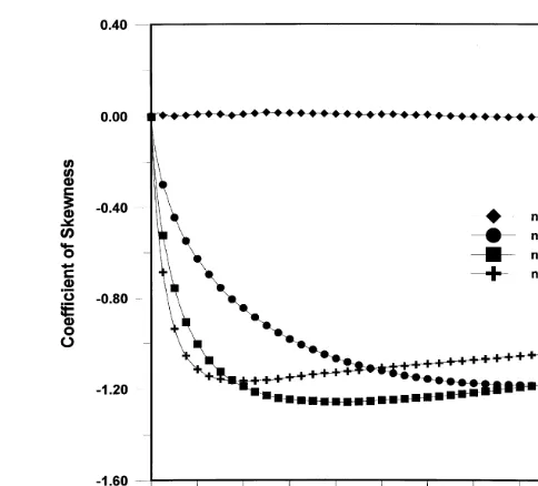
Finally the skewness coefficient of the plume is shown in Fig. 9. Since the plume for the linear case is symmetric, its skewness coefficient should be zero, which is what is seen from Fig. 9. However, for the nonlinear cases we observe that the solute plume is skewed to the left, which is indicated by the negative skewness coefficients shown in Fig. 9. It can also be seen that the absolute skewness coefficient is, for some time, larger for the smaller isotherm exponent, indi-cating a sharper front and longer tail relative to the size of the plume. However, as Fig. 9 shows, the skewness coeffi-cient tends to zero after a long time. This behavior is due to the tendency of the concentration gradients to vanish in the case of spatial uniformity of concentration. This behavior is also evidenced by the behavior depicted in Fig. 8(b) which shows the normalized peak concentration to asymptotically approach zero.
Another measure of skewness is the distance between the center of mass and the peak concentration, which is shown in Fig. 10. The behavior depicted in Fig. 10 was slightly smoothed by taking the 7-point average of the actual simu-lation results. It is seen from Fig. 10 that the center-of-mass to peak distance hovers around zero for the linear isotherm case, as expected since the plume is symmetric. For the nonlinear isotherms, however, it increases as the isotherm exponent decreases, attesting to the behavior that the front gets sharper and the tail flatter. Note the linear trend of the behavior in Fig. 10, indicating that the tail of the plume stretches at a steady rate.
Fig. 8. (a) Total mass in liquid phase normalized by initial injected mass. (b) Peak concentration normalized by initial peak
concentration.
5 DISCUSSION
This paper dealt with the simpler case of a hydraulically and chemically homogeneous flow domain. Other researchers have already presented results for more complicated flow domains. Tompson40considered flows in three-dimensional homogeneous and heterogeneous domains and a solute injected from an instantaneous point source. He evaluated simulated results from single long-term simulations in terms of plume center of mass velocity and plume spread variance. More recently Bosma et al.9 used the PTRW method to solve the transport equation for an instantaneously injected solute pulse. They used only 2000 particles to represent the solute plume and analyzed averaged spatial moments obtained from Monte Carlo simulations.
The results presented in this paper closely correspond to the results presented by Tompson40 for the case of the homogeneous domains. The behaviors of the plume center of mass velocity, plume spread variance, and skewness of plume concentration field presented in this paper are comparable to those illustrated by Tompson. In addition to the results presented by Tompson, we have demonstrated the sensitivity of the plume behavior to the isotherm expo-nent, which is in agreement with the findings of Bosma
et al.9
One problem with the current application of the PTRW method is the limited concentration resolution associated with using a fixed number of particles to represent the solute mass for cases of nonlinear sorption. This limitation was observed to influence the amount of tailing for the plumes. These tails should extend back to the injection point, but due to the limited concentration resolution the tails did not extend that far. To test the effect of particle numbers we have performed selected simulations with various numbers of particles, including 20 000, 100 000, 200 000 and 500 000
particles. We found that the greater the number of particles used, the greater is the amount of tailing. We also found that at small times, the simulations with 20 000 particles are identical to the results for 500 000 particles. However, as time increases the number of particles needed to provide accurate results increases. It is expected that at some suffi-ciently large time, even 500 000 particles will not provide adequate accuracy. As the number of particles used directly influences the computational demand for the simulation, it will be necessary to improve the computational efficiency of the PTRW method.
One improvement to the PTRW method would be to use an adaptive procedure where particles in regions with low particle numbers would be subdivided to increase concen-tration resolution. Such a procedure would allow a simula-tion to begin with a relatively small number of particles, and then the number of particles would be increased to auto-matically adapt to conditions of either low concentration or high concentration gradients. This should reduce the overall computation demand of a simulation.
6 SUMMARY AND CONCLUSIONS
In this paper the Particle Tracking Random Walk method has been implemented for the simulation of the transport of sorbing solutes with nonlinear equilibrium isotherms in a homogeneous flow field. Numerical experiments were performed to study the effects of the nonlinearity of the sorption isotherm on the behavior of the plume of a sorbing solute. The flow field was a saturated two-dimensional rectangle with constant mean flow velocity in one direction. The numerical experiments consisted of releasing 200 g of solute as a pulse and tracking their movements using 200 000 particles to represent the solute mass. The Freun-dlich isotherm exponents examined varied between 0.7 and 1.0. Results were presented in terms of the plume center-of-mass velocity, spread variance, skewness, and breakthrough curves. Findings of the study can be summarized as follows:
1. As the plume spreads the velocity of its center-of-mass decreases because of the increased retardation caused by decreasing concentrations. The decrease in the velocity was observed to be fastest at earlier times due to a larger initial decrease of the concentrations. The plume was observed to move faster for smaller values of the Freundlich isotherm exponent at earlier times, but the order was reversed at large times. 2. Except for the symmetric case of the linear isotherm
(n¼1.0), the plume was observed to develop a long tail due to the differential retardation behavior. Theoretically the tail should extend back to the point of injection because, according to the Freund-lich isotherm, the retardation coefficient tends to infinity in the limit as the liquid concentration approaches zero. The implication of this is that once a site is invaded by a contaminant that obeys the Fig. 10. Distance between plume center of mass and peak
Freundlich isotherm, it would be impossible to clean it completely.
3. The advancing front of the solute was seen to get sharper as the plume advanced, again due to the behavior of the retardation coefficient rapidly increas-ing across the front of the plume.
4. While advancement of the solute front was hindered by the nonlinear sorption, the spread variance was found to increase nonlinearly with time. Nonlinearity was stronger for smaller isotherm exponents. The increase in the spread variance is primarily due to the stretching tail behind the plume, not to increased spreading at the front. This is because the variance is related to the square of the distance from the center of mass.
5. Due to the long tail and the sharp front of the plume the skewness was found to be negative and its abso-lute value increasing with time for nonlinear isotherms; for linear isotherms the plume was symmetric. At large times the trend of the absolute skewness was found to reverse and tended to zero, which is due to the flattening of the tail and vanishing of concentration gradients. It was observed that the more nonlinear the isotherm, the stronger the trend toward zero.
ACKNOWLEDGEMENTS
Published as Paper No. 22,585 of the scientific journal series of the Minnesota Agricultural Experiment Station on research conducted under Minnesota Agricultural Experi-ment Station Project No. 12-047. This work was partially supported by the Army High Performance Computing Research Center under the auspices of the Department of the Army, Army Research Laboratory cooperative agree-ment number DAAH04-95-2-0003/contract number DAAH04-95-C-0008, the content of which does not neces-sarily reflect the position or the policy of the government, and no official endorsement should be inferred. Additional support for numerical simulations was provided by the Uni-versity of Minnesota Supercomputer Institute.
REFERENCES
1. Abulaban, A., Modeling the transport of sorbing solutes in heteroge-neous porous media. Ph.D. dissertation, Dept. Civil and Mineral Engi-neering, University of Minnesota, Minneapolis, Minnesota, 1993. 2. Ahlstrom, S. W., A mathematical model for predicting the transport
of oil slicks in marine waters. Battelle, Pacific Northwest Labora-tories, WA, 1975.
3. Ahlstrom, S. W., Foote, H., Arnett, R., Cole, C. and Serne, R., Multi-component mass transport model: Theory and numerical implementa-tion. Report BNWL 2127, Battelle Pacific Northwest Laboratories, Richland, WA, 1977.
4. Allen, C. M. Numerical simulation of contaminant dispersion in estuary flows. Proc. Roy. Soc. London A, 1982, 381 179–194. 5. Bear, J. On the tensor form of dispersion in porous media. J. Geophys.
Res., 1961, 66 1185.
6. Bear, J., Dynamics of Fluids in Porous Media. Elsevier, New York, 1972, 764 pp.
7. Bork, I. & Maier-Reimer, E. On the spreading of power plant cooling water in the tidal river applied to the River Elbe. Adv. Water Resour., 1978, 1 161–168.
8. Bosma, W. J. P. & van der Zee, S. E. A. T. M. Dispersion of a continuously injected, nonlinearly adsorbing solute in chemically or physically heterogeneous porous formations. J. Cont. Hydrol., 1995,
18 181–198.
9. Bosma, W. J. P., van der Zee, S. E. A. T. M. & van Dujin, C. J. Plume development of a nonlinearly adsorbing solute plume in heteroge-neous porous media. Water Resour. Res., 1996, 32 1569–1584. 10. de Marsily, G., Quantitative Hydrogeology, Groundwater Hydrology
for Engineers. Academic Press, New York, 1986.
11. Faust, C. R. & Mercer, J. W. Groundwater modeling: Recent devel-opments. Ground Water, 1980, 18 569–577.
12. Gardiner, C. W., Handbook of Stochastic Methods for Physics, Chem-istry and the Natural Sciences, 2nd edn. Springer-Verlag, Berlin, 1985.
13. Gasser, R. P. H., An Introduction to Chemisorption and Catalysis by Metals. Oxford University Press, New York, 1985, 260 pp. 14. Gillham, R. W., Cherry, J. A. and Pickens, J. F., Mass transport in
shallow groundwater flow systems. In Proceedings of the Canadian Hydrology Symposium. National Research Council of Canada, Ottawa, Canada, 1975, pp. 361–369.
15. Hamaker, J. W. and Thompson, J. M., Adsorption. In Organic Chemicals in the Soil Environment, ed. C. M. Goring and J. W. Hamaker. Marcel Dekker, New York, 1972.
16. Healy, R. W. & Russel, T. F. A finite-volume Eulerian–Lagrangian localized adjoint method for solution of the advection–dispersion equation. Water Resour. Res., 1993, 29 2399–2413.
17. Heller, J. P., Observations of mixing and diffusion in porous media. In Proceedings of the Second International Symposium on Funda-mentals of Transport in Porous Media. IAHR, Guelph, Canada, 1972, pp. 1-26.
18. Hunter, J. R., Numerical simulation of currents in Koombana Bay and the influence of the new power station. Environmental Dynamics Report ED-83-049, University of Western Australia, 1983. 19. Hunter, J. R., The application of Lagrangian particle tracking
techniques to modeling of dispersion in the sea. In Numerical Model-ing: Application to Marine Systems, ed. J. Noye. Elsevier Science Publishers B.V. (North-Holland), Amsterdam, The Netherlands, 1987.
20. Kinzelbach, W., Groundwater modeling. Developments in Water Science 25. Elsevier, Amsterdam, The Netherlands, 1986.
21. Kinzelbach, W., The random walk method in pollutant transport simulation. In Groundwater Flow and Transport Modeling, ed. E. Custodio, A. Gurgui and J. P. Lobo Ferreira. D. Riedel, Dordrecht, The Netherlands, 1988.
22. Kinzelbach, W. and Schafer, W., Coupling of chemistry and trans-port. In Groundwater Management: Quantity and Quality, Proceed-ings of the Benidorm Symposium, ed. A. Sahuquillo, J. Andreu and T. O’Donnell, October, 1989. IAHS publ. #188, Wallingford, UK, 1989, pp. 237–260.
23. McCarty, P. L., Reinhard, M. & Rittman, B. E. Trace organics in ground water. Envir. Sci. Technol., 1981, 15 40–51.
24. Nieber, J. L. & Walter, M. F. Two-dimensional soil moisture flow in a sloping rectangular region: Experimental and numerical studies. Water Resour. Res., 1981, 17 1722–1730.
25. Noye, B., Time-splitting the one-dimensional transport equation. In Numerical Modelling: Applications to Marine Systems, ed. B. J. Noye. Elsevier Science Publishers B.V., Amsterdam, 1986, pp. 271–295.
26. Pinder, G. F. Groundwater contaminant transport modeling. Envir. Sci. Technol., 1984, 18 108A–114A.
28. Rao, P. S. and Jessup, R. E., Sorption and movement of pesticides and other toxic organic substances in soils. In Chemical Mobility and Reactivity in Soil Systems, Proceedings of a Symposium Sponsored by Divisions S-1, S-2 and A-5 of the American Society of Agronomy and the Soil Science Society of America, ed. D.W. Nelson, D. E. Elrick and K. K. Tanji, Atlanta, GA, 29 November–3 December, 1981. SSSA special publ. #11, Madison, Wisconsin, USA, 1983. 29. Risken, H., The Fokker–Planck Equation. Springer-Verlag, Berlin,
1984.
30. Scheidegger, A. E. Statistical hydrodynamics in porous media. J. Appl. Phys., 1954, 25 994.
31. Schwartz, F. W. Macroscopic dispersion in porous media: The con-trolling factors. Water Resour. Res., 1977, 13 743–752.
32. Simpson, E. S. A note on the structure of the dispersion coefficient. Geol. Soc. Amer. Abs. Program, 1978, 10 493.
33. Smith, L. & Schwartz, F. W. Mass transport, 1. A stochastic analysis of macroscopic dispersion. Water Resour. Res., 1980, 16 303–313. 34. Smith, L. & Schwartz, F. W. Mass transport, 1. Analysis of
uncer-tainty in prediction. Water Resour. Res., 1981, 17 351–369. 35. Sposito, G., The Surface Chemistry of Soils. Oxford University Press,
New York, 1984, 234 pp.
36. Su, N. Development of the Fokker–Planck equation and its solu-tions for modeling transport of conservative and reactive solutes in physically heterogeneous media. Water Resour. Res., 1995, 31 3025–3032.
37. Tompson, A. F. B., Vomvoris, E. A. and Gelhar, L. W., Numerical simulation of solute transport in randomly heterogeneous porous media: Motivation, model development and application. Report #36, Ralph M. Parson Laboratory, Dept. of Civil Eng., Mass. Inst. of Tech., Cambridge, MA, 1988.
38. Tompson, A. F. B. & Gelhar, L. W. Numerical simulation of solute transport in three-dimensional randomly heterogeneous porous media. Water Resour. Res., 1990, 26 2541–2562.
39. Tompson, A. F. B. & Dougherty, D. E. Particle-grid methods for reacting flows in porous media with application to Fisher’s equation. Appl. Math. Model., 1992, 16 374–383.
40. Tompson, A. F. B. Numerical simulation of chemical migration in physically and chemically heterogeneous porous media. Water Resour. Res., 1993, 29 3709–3726.
41. Uffink, G. J. M., A random walk method for the simulation of macro-dispersion in a stratified aquifer. In Relation of Groundwater Quality and Quantity, Proceedings IUGG–IAHS Symposium in Hamburg, ed. F. X. Dunin, G. Matthess and R. A. Gras. IAHS Publ. #146, Wallingford, Oxfordshire, UK, 1985, pp. 103–114.
42. Uffink, G. J. M., Modeling of solute transport with the random-walk method. In Groundwater Flow and Transport Modeling, ed. E. Custodio, A. Gurgui and J. P. Lobo Ferreira. D. Riedel, Dordrecht, The Netherlands, 1988.
43. Valocchi, A. J. Spatial moment analysis of the transport of kinetically adsorbing solutes. Water Resour. Res., 1989, 25 273–280. 44. Van Kampen, N. G., Stochastic Processes in Physics and Chemistry.
North-Holland Publishers, Amsterdam, The Netherlands, 1981. 45. Vomvoris, E. G., Concentration variability in transport in heterogeneous
aquifers: A stochastic analysis. Ph.D. dissertation, Dept. of Civil Engi-neering, Massachusetts Institute of Technology, Cambridge, MA, 1986. 46. Vomvoris, E. G. & Gelhar, L. W. Stochastic analysis of the concen-tration variability in three-dimensional heterogeneous aquifers. Water Resour. Res., 1990, 26 2591–2602.
47. Warren, J. E. & Skiba, F. F. Macroscopic dispersion. Soc. Petrol. Eng. J., 1964, 4 215–230.
48. Weber, W. J. Jr, McGinley, P. M. & Katz, L. E. Sorption phenomena in subsurface systems: Concepts, models, and effects on contaminant fate and transport. Water Res., 1991, 25 499–528.