RADIOMETRIC CALIBRATION OF TLS INTENSITY:
APPLICATION TO SNOW COVER CHANGE DETECTION
K. Anttila a,b, *, S. Kaasalainen a, A. Krooks a, H. Kaartinen a, A. Kukkoa, T. Manninen b, P. Lahtinen b, and N. Siljamo b a
Finnish Geodetic Institute, Geodeetinrinne 2, P.O. Box 15, FI-02431 Masala, Finland. (e-mail [email protected]) b
Finnish Meteorological Institute, Earth Observations, P.O. Box 503, FIN-00101 Helsinki, Finland
Commission VI, WG VI/4
KEY WORDS: Terrestrial Laser Scanning, Radiometric Calibration, Snow Cover, Topographic Effect
ABSTRACT:
This paper reports on the radiometric calibration and the use of calibrated intensity data in applications related to snow cover monitoring with a terrestrial laser scanner (TLS). An application of the calibration method to seasonal snow cover change detection is investigated. The snow intensity from TLS data was studied in Sodankylä, Finland during the years 2008-2009 and in Kirkkonummi, Finland in the winter 2010-2011. The results were used to study the behaviour of TLS intensity data on different types of snow and measurement geometry. The results show that the snow type seems to have little or no effect on the incidence angle behaviour of the TLS intensity and that the laser backscatter from the snow surface is not directly related to any of the snow cover properties, but snow structure has a clear effect on TLS intensity.
* Corresponding author.
1. INTRODUCTION
The radiometric calibration of laser scanner intensity should comprise a sequence of corrections that convert the instrumental (raw) intensity information into a value proportional or equal to target reflectance. The intensity information produced by current commercial TLS instruments is mostly meant to enhance the range determination, so it is often strongly modified by the instrument, requiring some extra calibration steps. Even though the intensity data acquisition is never optimized, the use of the TLS intensity data is increasing, and there is a greater need for radiometric calibration methods. Studies on the TLS intensity and calibration methods have been proposed quite recently (Pfeifer et al. 2008, Kaasalainen et al., 2009a, Balduzzi et al., 2011).
Using terrestrial laser scanning (TLS) in snow cover monitoring has originated from the growing interest in remote monitoring in, e.g., boreal or alpine regions because of the inaccessibility of these regions and the complications they cause for traditional observation methods. Long-range laser scanners (up to 2500 m) are usually preferred for this purpose and tested, for example, in measuring snow depth and in profiling avalanche hazard regions (Prokop, 2008, Schaffhauser et al., 2008). Comparison and synchronous use of TLS with other methods such as tachymetry, SAR, and manual probing has shown that TLS is a quick means of getting high-density point data (Prokop et al., 2008). In particular, TLS has major advantages over manual probing, which is often time consuming and dangerous. The integration of TLS and microwave ground-based synthetic aperture radar (SAR) data has also been studied for measuring the snow depth in mountainous regions (Luzi et al., 2009). The first applications of laser scanner intensity data in glaciology, together with point cloud data, have mostly been related to target classification in glaciers (Höfle et al., 2007). Snow cover
plays a crucial role in the determination of Earth’s surface
albedo, which is an important climate parameter (e.g., Køltzow, 2007). Seasonal changes in the snow cover are closely related to
water cycle and winter warming in the boreal zone. Snow cover also strongly impacts climate in the arctic region and affects, for example, the length of the growing season (Bokhorst et al., 2009).
We have developed a radiometric calibration scheme for airborne laser scanning (ALS) intensity data, based on the use of external reference targets, for which the reflectance is measured in a laboratory or in situ. This calibration method was extended to TLS (Kaasalainen et al., 2009a). In this paper, we present an application of TLS intensity calibration to studying the seasonal snow cover brightness and change detection from TLS range and intensity data. This is particularly important in a forested environment, where surface visibility for airborne laser and satellite data is limited. TLS could provide a cost-effective and multi-temporal approach for gaining information and data on these environments for applications like fractional snow cover mapping. This study is also related to satellite validation efforts as part of a multi-scale approach for the improved characterization of snowmelt patterns in boreal regions: the Snow Reflectance Transition Experiment (SNORTEX) is part
of SAF’s (Satellite Application Facilities) Land, Climate and
Hydrology activities, which are supported by EUMETSAT and meteorological institutes (Roujean et al., 2010).
2. METHODS
2.1 The Study Sites
In order to investigate the use of TLS intensity data in snow monitoring we made several TLS measurements during the SNORTEX 2009 field campaign in Sodankylä (67.4 °N, 26.6 °E) using the existing facilities provided by FMI-ARC (the Finnish Meteorological Institute, Arctic Research). The test site was located in the vicinity of the FMI-ARC research station (Tähtelä).The campaign took place during the snow-melt season, which lasts from March through May. The
measurements included stationary TLS measurements made in one given location and repeated in different days. In addition to TLS data, we observed the air temperature and overall weather and snow conditions. The approximate air temperature was measured with a non-calibrated thermometer of a car in order to get values for the days without calibrated thermometer measurements (28th April and 29th April). To study the topographic effect for different snow types, we carried out a time series of incidence angle measurements. These measurements were made in Masala, Kirkkonummi (Sourthern Finland, 30 km west from Helsinki) during Dec 2010- Jan 2011.
2.2 Terrestrial Laser Scanning in Sodankylä
Leica HDS6000 terrestrial laser scanner was used for the measurements in 2009 in Sodankylä. It employs a continuous wave of 650-690 nm. The scanner uses phase modulation with three different carrier wavelengths and an unambiguity range of approximately 79 metres, for the distance measurement. The distance measurement accuracy is 4-5 mm. The field-of-view is 360° × 310°, the circular beam diameter at the exit is 3 mm and the beam divergence is 0.22 mrad. The Leica scanner also has an angular resolution that can be selected between 0.009° and 0.288°. The scanner uses a silicon Avalanche Photo Diode (APD) as a photo detector. Later the HDS6000 was updated to HDS6100, which was used in Masala in 2010-2011.
We georeferenced the different Tähtelä measurements using common points, i.e. targets such as details in tree trunks that could be identified in each point cloud. This way the laser scans from several days were transformed into the same reference frame of the first measurement and all the measurements could be compared as a time series. In this way we could also obtain the intensity values from the same sample plots for all the measurements. TLS profile snow depth for each day was computed by making another scan during summer with no snow present putting the datasets in same reference frames, cutting profiles from the laser data and calculating the distance between the winter and summer profiles.
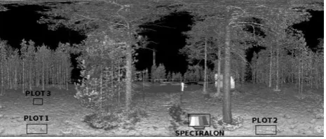
Using the laser intensity image, we selected 3 representative eliminated the effects of distance and the incidence angle while comparing the different measurements.
The first two plots were located at a distance of approximately 2 metres and the third plot about 5 metres from the scanner. By comparing the measurements at the same distance and incidence angle, we could minimize the topographic and distance effects on the time series. For our time series, we used the average intensity value of each plot separately.
The size of the sample plots was about 0.7m x0.7 m. Plots 1 and 2 consisted of approximately 200 000 points and plot 3 of 70 000 point. The number of points in the Spectralon panel plots varied from 5000 to 15000 points between different TLS measurements. The calibrated intensity for each plot is the mean intensity value of all the laser points inside the plot, divided by the mean intensity of the Spectralon. The standard deviations (normalized values) of plots 1, 2 and 3 were between 3% and
5% with 3% being the most common value. For the Spectralon panel the values for standard deviation were around 1%.
Fig. 1. Intensity image of a measurement from Tähtelä. The square plots 1, 2 and 3 are the sample plots and the Spectralon is the reference panel.
The intensity values for the Leica HDS6000 scanner have been found to be linear, and no logarithmic corrections are needed. This requires the use of Z+F LaserControl 7.4.5 (Zoller+Fröhlich GmbH) software for the extraction of raw intensity instead of the Leica Cyclone 6 software, where normalizing and data pre-processing destroy the linearity (see Kaasalainen et al., 2009a for more details).
The intensity calibration was carried out using a Spectralon measurement, so we corrected the values for the incidence angle effect to correspond to the values of a Spectralon perpendicular to the incoming laser beam: both horizontal and vertical incident angles were calculated from Spectralon surface normal vector derived from the point cloud.
2.3 Incidence Angle Measurements in Masala
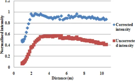
The role of topographic (incidence angle) and distance effects in the radiometric calibration of terrestrial laser scanner data has been previously investigated by Kukko et al. (2008) and Kaasalainen et al. (2009a, 2009b). The distance effect for the Leica scanner (also used in this experiment) has been studied in Kaasalainen et al. (2009a). For the first 5 metres, the intensity is reduced to keep the intensity level within the sensor dynamic range. From 5 metres and beyond the intensity function follows roughly the 1/r2 rule where r is the range of the laser beam. The Leica HDS 6000 stores intensity correction values in 1 metre interval to its scan file headers and rudimentary automatic correction of the intensity values is possible by using Z+F LaserControl (Zoller+Fröhlich GmbH) software. The automatic correction works best with distances between 2 to 10 metres (Figure 2).
To study the topographic effect for different snow types, we carried out a time series of incidence angle measurements. The aim was to investigate if the incidence angle behaviour for different snow types follow the cosine law (see, e.g., Kaasalainen et al., 2009b). These measurements were made in Masala, Kirkkonummi (Sourthern Finland) during Dec 2010- Jan 2011, also using Leica HDS 6000. A flat snow surface was measured on the rooftop at different weather conditions (e.g.,
air temperatures ranging from -14C to +1.5C, the snow conditions varying from fresh dry snow to wet (rounded) grains. The data was corrected for distance similarly to Fig. 2. The 99% Spectralon panel was used for intensity calibration. The distance range in these measurements was from 2 to 26 meters.
Figure 2. The effect of Z+F LaserControls distance correction on TLS intensity values (of the 99% Spectralon
panel). The raw intensity values have been normalised to a scale of 0 to 1.
2.4 Ground Reference in Sodankylä
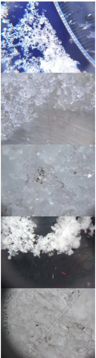
To study the effect of snow grain size and structure on the TLS intensity, we took images of the snow crystals using a Canon Powershot pocket camera attached to a magnifier loupe with a 0.1 mm scale. The snow cover depth was also measured during a snow pit measurement, which was carried out in the late afternoon on each day that TLS measurements were made except for the last two snow-pit measurements, which were done in the morning. The exact measuring time depended on the schedule of all the field measurements during the day. The snow depth was measured with a stick in three places near the pit and the average from these values was used as the snow depth. Other parameters, such as the Snow Water Equivalent (SWE), and temperatures of the snow surface and air were recorded during the snow pit experiments. In addition to these procedures, the weather station at the Tähtelä Observatory (FMI-ARC) automatically takes air temperature and wind speed measurements and the snow depth is constantly monitored by an automatic snow depth sensor.
3. RESULTS
We compared the backscattered reflectance of the snow samples with different weather and snow properties such as air temperature, snow depth, snow density, snow water equivalent (SWE is a measure of the amount of the water stored in a snowpack per unit of area, expressed in units of length, for example millimetres), surface temperature, temperature from the top layers of the snow pack and crystal size and shape for every measurement site. The results are presented in Figs. 3-5. Changes in the snow pack affect the intensity values of TLS, but none of the single parameters (air/surface temperature, SWE, snow density, snow depth) had a direct effect on the intensity. Instead, the backscattered intensity appears to be mainly related to crystal structure (Fig. 6) and the brightness (optical brightness and impurities) of the surface of the snow pack. During the first measuring day, the snow was dry. After this, the snow began to melt and the intensity values were considerably
lower. The intensity shows a clear peak on April 28th, even though the snow depth increased only a little due to snowfall. The snowfall in Apr 28 is also seen in the snow surface profile taken from the TLS point cloud data (Fig. 7). Because of the new snow, there was a change in the crystal structure of the snow surface (see Fig. 6). Since the old snow below the new layer was already melting, the new snow started melting fast and the intensity values dropped again on April 29th.
12th March 2009
FGI TLS laser FMI-ARC laser point manual
Sn
Figure 3. Snow depth measured manually (with snow stick), snow depth sensor measurements (FMI-ARC) and
TLS profiles at Tähtelä. The laser point measurements were made at different location than
the other measurements.
snow depth laser (cm) snow1 (norm) snow2 (norm) snow3 (norm)
Sn
Figure 4. The calibrated TLS intensity (backscattered reflectance) and snow depth (measured with TLS) at
the Tähtelä measurement site. The intensity (backscattered reflectance) scale is on the right of
the plot.
Figure 5. The air and surface temperatures and intensities of the 3 sample plots in Tähtelä in different days. For 28th
April and 29th April approximate air temperatures were used. They had no connection to the
backscattered reflectance.
Figure 6. The images of the snow of the following dates (top down): 12th March 2009, 23rd, 27th, 28th, and 29th April 2009, showing the change in crystal structure in April 28. The millimetre scale is visible in the
highest and lowest images.
Figure 7. The snow surface profiles from Tähtelä at each date of laser scanning. Each profile represents the snow surface height of one measurement. The Summer 2008 measurement represent the ground level. The
scanner is at the coordinates 0,0.
The calibrated intensities of plots 1 and 2 (the intensity at each test plot is shown in the graphs in Figs. 4 and 5) reacted more strongly to the changes in the snow crystals and brightness than the intensity of plot 3, which was further away from the laser scanner. This is because the distance effect causes the intensities to decrease further from the scanner. An increase in the incidence angle also decreases the intensity values, which decreases the relative effect of the surface properties. The effect of incidence angle on TLS intensity from snow is presented in Fig. 8 for different snow types. There is large variation in both air temperatures and snow grain properties between each date: snow grain size ranging from 0.5 mm to several millimetres, and the grain shapes from hexagonal (Nov 22) to strongly rounded an aggregated grains at the wet conditions (Jan 10, Jan 18). While the intensity in wet conditions (Jan 10 and Jan 18 measurements) appears slightly lower, the effect of incidence angle does not show a strong dependence on snow grain properties (and hence the snow type). More data including measurements with smaller incidence angles is needed to better understand the effect of incidence angle on the intensity of the laser backscattering from different snow surfaces.
Figure 8. The normalized intensity of the incidence angle measurements. The air temperatures at each day were: Nov 22: -7°C (new snow), Nov 30: -13.9°C, Dec 2: -2.5°C (rounded grains), Jan 10: +1.5°C (wet
snow), Jan 18: +0.6°C (wet snow, recent rainfall). The field of view of the scanner is 25°-335°.
4. CONCLUSION
We have studied the radiometric calibration of TLS intensity data in applications related to snow cover monitoring with TLS, and investigated the usability of TLS intensity in environmental applications. The reflected surface intensity values depend on the snow characteristics in a complex way, so that no single parameter (snow cover thickness, temperature, grain size, etc.) has a clear relationship with it. The crystal shape and surface albedo had the strongest effect on the laser intensity: the rounded crystal structure of old and melting snow produced significantly lower intensities than new snow with sharp crystals, which showed clear peaks in intensity. The results agree with earlier findings (e.g., Prokop, 2008). An interesting feature is that the snowpack properties seem to have little effect on the topographic (incidence angle) effect on TLS intensity. This might enable a similar correction of incidence angle effects for all snow types, but these results will be further analyzed together with a more detailed study of the topographic effect on TLS intensity data for different targets. Since calibrating the incidence angle and distance effects on snow surface seems straightforward it further encourages the use of the intensity values alongside range data in snow surface applications.
The calibrated intensity features could be used together with range data to detect changes in the snowpack, i.e. to monitor the melt and distinguish between covered and snow-free areas, especially towards the end of the melting process.
While these results are preliminary, and the methods need to be further investigated, the results indicate that calibrated intensity data enhances the use of TLS for snow surface monitoring. Even though the measurement of TLS intensity is not likely to be optimized in the near future, this study provides some practical steps towards the correction, feasibility, and limits in the application of intensity information as a side product of TLS range measurement. As the usage of TLS intensity data is constantly increasing, a practical approach to its correction is also needed.
5. REFERENCES
Balduzzi, M.A.F., Van der Zande, D., Stuckens, J., Verstraeten, W.W., and Coppin, P., 2010. The Properties of terrestrial laser system intensity for measuring leaf geometries: a case study with conference pear trees (Pyrus Communis). Sensors, 11(2), pp. 1657-1681.
Bokhorst, S. F., Bjerke, J. W., Tømmervik, H., Callaghan, T. V. and Phoenix, G. K., 2009. Winter warming events damage sub-Arctic vegetation: consistent evidence from an experimental manipulation and a natural event. Journal of Ecology, 97(6), pp. 1408-1415.
Höfle, B., Geist, T., Rutzinger, M., and Pfeifer, N., 2007. Glacier surface segmentation using airborne laser scanning point cloud and intensity data. Proceedings of ISPRS Workshop Laser Scanning SilviLaser. International Archives of Photogrammetry and Remote Sensing, Vol. XXXVI, part 3/W52, pp. 195-200.
Kaasalainen, S., Krooks, A., Kukko, A., and Kaartinen, H., 2009a. Radiometric Calibration of Terrestrial Laser Scanners
with External Reference Targets. Remote Sensing, 1(3), pp. 144-158.
Kaasalainen, S., Vain, A., Krooks, A., and Kukko, A., 2009b. Topographic and distance effects in laser scanner intensity correction. International Archives of Photogrammetry, Remote Sensing and Spatial Information Sciences, Paris, France, Vol. XXXVIII, part 3/W8, pp. 219-223.
Køltzow, M., 2007 The effect of a snow and sea albedo scheme on regional climate model simulations. Journal of Geophysical Research, 112(D07110), doi: 10.1029/2006JD007693. terrestrial laser scanner to monitor a snow-covered slope: results from an experimental data collection in Tyrol (Austria). IEEE Transactions on Geosciences and Remote Sensing, 47(2), pp. 382-393.
Pfeifer N., Höfle B., Briese C., Rutzinger M., and Haring A., 2008. Analysis of the backscattered energy in terrestrial laser scanning data. In: International Archives of Photogrammetry, Remote Sensing and Spatial Information Sciences, vol. XXXVII, Part B5, pp. 1045-1052.
Prokop, A., 2008. Assessing the applicability of terrestrial laser scanning for spatial snow depth measurements. Cold Regions Science and. Technology. 54(3), pp. 155-163.
Prokop, A., Schirmer, M., Rub, M., Lehning, M. and Stocker, M., 2008. A comparison of measurement methods: terrestrial laser scanning, tachymetry and snow probing for the determination of the spatial snow-depth distribution on slopes. Annals of Glaciology, 49(1), pp. 210-216.
Roujean, J.-L., Manninen, T., Kontu, A., Peltoniemi, J., Hautecoeur, O. Riihelä, A., Lahtinen, P., Siljamo, N., Lötjönen, M., Suokanerva, H., Sukuvaara, T., Kaasalainen, S., Aulamo, O., Aaltonen, V., Thölix, L., Karhu, J., Suomalainen, J., Hakala, T. and Kaartinen, H., 2010. SNORTEX (Snow Reflectance Transition Experiment): Remote sensing measurement of the dynamic properties of the boreal snow-forest in support to climate and weather forecast. Report of IOP-2008. Proceedings of IGARSS 2009. Finland (project "New techniques in active remote sensing: hyperspectral laser in environmental change detection") and by the EUMETSAT Hydro-SAF project. The authors are grateful to the staff members of FMI-ARC.