INFORMATION-DRIVEN AUTONOMOUS EXPLORATION FOR A VISION-BASED MAV
Emanuele Palazzolo, Cyrill Stachniss
Institute of Geodesy and Geoinformation, University of Bonn, Germany {emanuele.palazzolo, cyrill.stachniss}@igg.uni-bonn.de
KEY WORDS:Exploration, Information Gain, MAV, UAV, Vision, Mapping
ABSTRACT:
Most micro aerial vehicles (MAV) are flown manually by a pilot. When it comes to autonomous exploration for MAVs equipped with cameras, we need a good exploration strategy for covering an unknown 3D environment in order to build an accurate map of the scene. In particular, the robot must select appropriate viewpoints to acquire informative measurements. In this paper, we present an approach that computes in real-time a smooth flight path with the exploration of a 3D environment using a vision-based MAV. We assume to know a bounding box of the object or building to explore and our approach iteratively computes the next best viewpoints using a utility function that considers the expected information gain of new measurements, the distance between viewpoints, and the smoothness of the flight trajectories. In addition, the algorithm takes into account the elapsed time of the exploration run to safely land the MAV at its starting point after a user specified time. We implemented our algorithm and our experiments suggest that it allows for a precise reconstruction of the 3D environment while guiding the robot smoothly through the scene.
INTRODUCTION
A common problem in autonomous 3D reconstruction is the se-lection of the viewpoints to cover the environment with the robot’s sensors in order to obtain a high-quality 3D model. This problem is often referred to as exploration. Micro aerial vehi-cles (MAVs) are becoming increasingly popular for 3D mapping due to their small size, low weight, and high mobility. On the downside, MAVs can carry only limited payloads and thus are often equipped with cameras instead of a typically heavier 3D laser scanner. Moreover, the overall weight of the platform limits its flight time and thus range as more energy is needed to carry the payload.
Typical autonomous exploration systems usually seek to mini-mize traveled distance, to cover as large as possible parts of the space, to actively reduce uncertainty, or other objectives (Fraun-dorfer et al., 2012; Forster et al., 2014; Mostegel et al., 2014; Schmid et al., 2012). In particular, the way the expected reduction of uncertainty is computed impacts the computational demands of the robot and strongly depends on the sensor setup. When it comes to MAVs operating in outdoor environments, they are often flown manually by a pilot as most countries require either manual flight or a continuous supervision of the MAV through an operator. From our experience, we found out that for an opera-tor, it is helpful if the MAV moves along a trajectory that is free of abrupt changes of direction. Moreover, due to its limited flight time the MAV needs a trajectory that allows it to land safely when running out of battery. Thus, an autonomous exploration system for MAVs should take such objectives into account when gener-ating flight trajectories.
As the main contribution of this paper, we propose an autono-mous exploration approach for MAVs that takes the above men-tioned objectives into account when selecting the next viewpoint for perceiving the object to be explored. In our setup, the user specifies the bounding box that contains the object of interest, for example a building that should be explored, and a time limit. Then, our algorithm makes its decisions according to a utility function, which focuses on reducing the uncertainty in the 3D
model and on producing a flight path with a small number of abrupt turns, while allowing a safe landing at the starting point within a given time constraint. We sample the possible next-best-views on a hull that initially surrounds the bounding box and then is iteratively refined to fit the explored building. We compute an approximation of the expected uncertainty reduction by taking into account the properties of the camera used for reconstruc-tion. To do so, we discretize the space into voxels and consider the uncertainty reduction in every voxel that contains measured points. Furthermore, our approach prefers paths that avoid abrupt turns in the flight direction to simplify the supervision of a hu-man operator. Moreover, a time dependent cost function supports a safe landing, preventing the MAV from flying above obstacles, reducing progressively its altitude and pushing it towards its start-ing point. We implemented our approach in C++ usstart-ing ROS and tested it in simulation as well as in a real indoor environment. Our experiments suggest that our algorithm yields a 3D reconstruction of the environment showing a low uncertainty in the probabilistic model and a trajectory with less changes of direction when com-pared to some of the current state-of-the-art algorithms used in an otherwise identical setup.
RELATED WORK
A common technique used for exploration is frontier-based ex-ploration, originally proposed by Yamauchi (1997). This ap-proach aims to choose the next viewpoint as the closest frontier between known and unknown areas in the map built so far. This approach is widely used and has been proven to be very effective in terms of reducing the path length of the robot. An example of its application to a MAV is the work of Fraundorfer et al. (2012), which keeps the MAV at a fixed altitude and explore the environ-ment by combining a traditional frontier-based exploration with a bug algorithm.
the problem for 2D mapping and exploration are the approaches Stachniss et al. (2005), or Perea Strom et al. (2015). When ex-ploring an environment, the aim is mostly a precise 3D recon-struction and the key problem is to select viewpoints that allow for that. This specific problem is also called view planning, next-best-view or active vision (Aloimonos et al., 1988; Bajcsy, 1988; Scott et al., 2003). A possible approach to this problem is pro-posed by Vasquez-Gomez et al. (2014), whose utility function balances unseen areas and overlaps with previous scans. An al-ternative is the method by Kriegel et al. (2011), which allows 3D reconstruction through the estimation of a surface, knowing only an approximate bounding box.
Most of these works, however, focus on the reconstruction of an object. Instead, we are typically interested in reconstructing a building or facade, which is not achievable by using, for example, a manipulator as done by Kriegel et al. (2011). The exploration of large buildings is addressed by Bircher et al. (2015). They use a Traveling Salesman Problem (TSP) solver on sampled points to compute at every iteration the shortest path for exploring a large structure with a MAV. This approach targets on coverage path planning, which is related but different from our problem, since it assumes a given triangular mesh of the building. In contrast, we only assume a general bounding box as initial model and refine it iteratively to improve the viewpoint selection. Another approach that focuses on 3D reconstruction with a MAV is the work by Schmid et al. (2012), who compute the views off-line by exploit-ing some previous knowledge about the environment, specifically a 2.5D model. To compute the path, they first select every not re-dundant viewpoint on a convex hull around the structure and then solve a TSP to minimize the path length. Related to the ques-tion where to look is also the quesques-tion, which landmark to use for effective mapping, see Strasdat et al. (2009).
Many other techniques have been used for exploration with MAVs, for example the work of Mostegel et al. (2014), who fo-cus more on localization stability rather than reconstruction, or the one by Sadat et al. (2014), whose path planning algorithm focus on maximizing feature richness. A particularly interesting approach is the one by Forster et al. (2014), which computes, sim-ilarly to us, the path by maximizing the information gain over a set of candidate trajectories, but in contrast to us, considers the texture of the explored surface.
Another relevant approach is the one by Charrow et al. (2015), which generates a set of trajectories by combining a frontier-based technique and local primitives generated by control sam-pling, then choose the one that maximizes the information-the-oretic objective and further optimize it with a gradient-based op-timization. Isler et al. (2016), instead, select the next-best-view according to the information gain in a volumetric map. They compute the information gain from different definitions of Vol-umetric Information, which represent the information enclosed in a voxel. Our approach is similar, but in contrast we include trajectory smoothness and elapsed time in the utility function and we compute the information gain as proposed by Pizzoli et al. (2014), enclosing that measurement uncertainty in the voxels.
Other noteworthy approaches are by Atanasov et al. (2015), who focus on decentralized multi-sensor information acquisition, and Freundlich et al. (2013), who plan the next-best-view to reduce the localization uncertainty of a group of stationary targets.
INFORMATION GAIN-BASED EXPLORATION
A frequently used approach for exploration is the frontier-based exploration, which considers the local space as either being ex-plored or unexex-plored. By guiding the robot to the closest frontier between the explored and the unexplored space, the robot itera-tively increases the explored area until the whole environment has been covered with the sensor’s field-of-view. The frontier-based approach can be seen as a simplified form of information gain-based exploration. By moving to and observing the unknown space, the robot acquires a certain amount of new information until the whole space is explored and no further information can be obtained.
Described more generally, information gain-based exploration seeks to select viewpoints resulting in observations that minimize the expected uncertainty of the robot’s belief about the state of the world. Throughout this work, we assume the pose of the UAV to be known. In practice, we use the pose estimate from a VO/IMU/DGPS combination as described in Schneider et al. (2016). LetS be the state of the world. We can describe the uncertainty of the belief aboutSthrough the entropyH(S):
H(S) =−
Z
p(S) lnp(S)dS. (1)
In order to estimate what amount ofnew informationwill be ob-tained by taking a measurementZwhile following the pathP from the current position to the viewpointP, we use the expected information gainI, also called mutual information, defined using the entropy as
I(S;ZP) =H(S)−H(S|ZP). (2)
The second term in Eq. (2) is the conditional entropy and is de-fined as
H(S|ZP) =
Z
p(z| P)H(S|ZP=z)dz. (3)
Unfortunately, reasoning about all potential observations or even observation sequences z in Eq. (3) is intractable in nearly all real world applications since the number of potential ments grows exponentially with the dimension of the measure-ment space and the number of measuremeasure-ments to be taken. Fur-thermore, the optimal solution will only be obtained if we take all possible sequences of viewpoints as a whole into account and not greedily select only the next viewpoint. As a result of that, most approaches stick to greedy exploration and it is also crucial to approximate the conditional entropy so that it can be computed efficiently. A suitable approximation, however, depends on the environment model, the sensor data, and the application so that no general one-fits-all solution is available.
In mobile robotics, one typically seeks to maximize the expected information gainIwhile minimizing the cost that is associated with actually recording the measurement. In most cases, this cost is assumed to be proportional to the distance that the robot has to travel or the time it takes to reachPfrom its current location, by following the pathP. This leads to a utility functionU, that can, for example, be specified by
Figure 1. The MAV’s movements are constrained to a hull (red dotted line) that is initially built around the user-specified bounding box (blue area), then is adapted according to the new explored (yellow squares) and unknown (gray squares) voxels.
so that the next viewpoint exploration problem turns into solving
P∗= argmax
P
U(P) (5)
whenever a new decision has to be made. The collision-free path Pcan be a simple straight line if there are no obstacles along it, or can be computed by a fast, low level path planner such as the one by Nieuwenhuisen and Behnke (2016).
INFORMATION-DRIVEN EXPLORATION FOR MAVS
Due to its capability of moving freely in 3D, a MAV is an at-tractive platform for mapping complex 3D scenes. In this paper, we target at autonomous exploration with a MAV with the goal of obtaining an accurate map of the scene. Since the problem of finding the optimal sequence of viewpoints for a complete explo-ration is NP-complete, it is hard to compute the optimal solution for an exploring MAV online. In order to apply the exploration approach with the available computational resources, we have to make approximations as explained in the following.
Restricting the Possible Viewpoints
First, we assume to have some a priori knowledge of the envi-ronment. We assume to know the bounding box of the space to explore, typically a bounding box that surrounds a building or similar object. We define a hull that initially surrounds the bound-ing box (see Figure 1) and we constraint the motion of the MAV to the hull. The hull is dynamically adapted to fit the explored building or object according to the map built so far (Figure 1). To simplify the view-point selection, we constrain the orientation of the MAV such that the sensor is always pointing towards the object. These assumptions allow us to reduce the dimensionality of the action space to a two-dimensional manifold and we can construct the search space by sampling possible viewpoints uni-formly on the hull. In our experiments, we sample 100 new points each time the next viewpoint has to be computed.
Measurement Uncertainty and Approximating the Informa-tion Gain
To express the uncertainty of the measured depth, we can directly exploit the formulation proposed by Pizzoli et al. (2014), which they used in their REMODE approach for computing the mea-surement uncertainty for two images. Given a pair of imagesIi
andIj, we compute the variance in the depth estimate of a 3D
pointxas
σj2= x
+ − kxk
2
, (6)
b
α β
+
d
a x
x+
β γ
Ii Ij
Pi Pj
Figure 2. The measurement uncertainty of a depth point from two images can be computed throughxandx+
as in the REMODE approach (Pizzoli et al., 2014) for 3D reconstruction
from monocular images.
I
I I
i
j k
P
Pj Pk
i
x x+
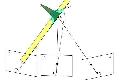
Figure 3. Illustration of the reduction of the uncertainty in the estimate about the 3D point location given a third image.
wherex+is obtained by back-projecting the uncertainty of mea-suring the pointxin the image plane from imageIj. Figure 2
shows an illustration of the estimation.
We need two views of a 3D point in order to obtain a Gaussian estimate. The uncertainty of the resulting Gaussian, directly de-pends on the angleγ. The closerγapproaches 90◦, the larger the uncertainty reduction.
The more views we add, the smaller the uncertainty becomes, i.e., any new observation of the point reduces its uncertainty, which is a part of the objective function of our exploration strategy. Fig-ure 3 illustrates this fact. After the first view with a monocular camera is available, we only know the direction of the point but not its depth, i.e., the uniform distribution shown in yellow. After the second view is obtained (or if a stereo camera is used), the Gaussian estimate shown in cyan is obtained. Further observa-tions, here illustrated through the imageIkreduce the uncertainty
further, see the dark green Gaussian.
Our aim is, therefore, to find the viewpoint that best reduces the uncertainty in the beliefs about all points. This uncertainty reduc-tion is given through the expected change in entropy. Thus, the mutual information for a Gaussian point estimate turns into
I(Sj;Zk) =
1 2ln
σ2
x,k+σ
2
x,j
σ2
x,k !
, (7)
whereZkrefer to the observations obtained at the camera
loca-tionPk, whileσx,j2 andσ
2
x,kare respectively the current
uncer-tainty of pointxfrom viewIjand the estimated uncertainty of
As a result of the Eq. (7), the expected uncertainty reduction that results from a new image depends on the current uncertainty of the point estimate and on the measurement uncertainty, which it-self depends on the geometric configuration of the new viewpoint with respect to the previous viewpoints.
Combining and Storing Information
To execute the above described approach on a MAV online during flight, we need an efficient way to store the information, which parts of the scene have been observed and from which viewpoints. To do that in an efficient manner, we compute a discretization of the 3D space covered by the bounding box of the environment to explore. This 3D discretization is maintained using octrees from the C++ library Octomap (Hornung et al., 2013) with a maximum resolution here set to0.125m3
, as we discretize the space into voxels with a size of0.5m×0.5m×0.5mand treat all points on one voxel alike, i.e., we compute the expected uncertainty re-duction per voxel only. Voxels that are still unexplored have the maximum uncertainty, as no information exists about the state of the cell.
As the correlation between the measurements is unknown, to combine the information from a new image with all the previous ones and compute the total uncertainty, we use the covariance in-tersection algorithm. Given two distributions of meansµ1,µ2
and covariance matricesΣ1,Σ2, it is possible to combine them in a third distribution of meanµ3and covariance matrixΣ3using the formulas:
whereωis a weighting parameter obtained typically by minimiz-ing the determinant or the trace ofΣ3. To computeω, we adopt the closed-form solution proposed by Reinhardt et al. (2012). We approximate the distribution resulting from two images to be uni-variate, assuming the uncertainty only on the depth of the point seen from the first image, which is, in turn, assumed without un-certainty.
Furthermore, we reduce the computational load by computing the covariance intersection only between each new view and the first 10 from which the point has been seen. The updated uncertainty is computed and stored for each voxel seen by the new image. As it is typical for occupancy grids, each voxel is assumed inde-pendent from the others, therefore the total entropy is the sum of the entropy of each voxel. Thus, the information gain of a view is the sum of the information gains of all the voxels seen by that view. Note that, since we acquire images at a constant framerate, for each candidate viewpoint we evaluate the information gain for all the intermediate images, by subsampling a computed path between the current position and the possible next one.
Changes of Flight Direction
Most exploration approaches ignore the shape of the trajectory. MAVs, however, often do not fly completely on their own as in most countries an operator must monitor the MAV during flight to take over control in case of problems. According to our experi-ence, an autonomous MAV with a too erratic motion substantially complicates the life of a safety pilot.
Thus, we are interested in a trajectory that, while maximizing the information gain and keeping the trajectory short, avoids sharp changes of direction and prefers a continuous motion. We can obtain such a behavior by defining the cost function as:
cost(P) =d(P) +θ(P), (10)
whered(P)grows linearly with the length of the pathPbetween the current location of the robot and pointP, whileθ(P)is a func-tion that grows linearly with the maximum change in orientafunc-tion that must be executed by the MAV along the path.
Time-Dependent Cost Function
At some point in time, a MAV runs out of battery. To prevent it from crashing or to reduce the impact of it, we add a time-dependent component to our cost function before the battery runs low. This critical time valuetcriticalis dynamically computed ac-cording to the trajectory needed to move the MAV to the starting point from the current location to enable a controlled landing. On our system, this trajectory is computed by a low-level plan-ner (Nieuwenhuisen and Behnke, 2016). Once the time-depen-dent cost function is enabled, it favors viewpoints for the MAV to:
• fly towards the starting point (for landing),
• avoid flying above obstacles to allow for a potential emer-gency landing, and
• fly closer to the ground to prevent possible impacts if the bat-tery dies.
Thus, we extend the cost function in Eq. (10) to:
cost(P, t) =d(P) +θ(P) +T(t)
• f(t)grows linearly with the elapsed time if the area below the MAV is not free, it is equal to0otherwise;
• dstart(t)grows linearly with the elapsed time and is
propor-tional to the distance between the current position and the starting point;
• z(t)grows linearly with the elapsed time and is proportional to the current altitude of the MAV.
These terms can be chosen in different ways. In our implementa-tion, we represent the cost function as a weighted sum of the dif-ferent terms, where the weights are tuned by hand. The functions
f(t),dstart(t)andz(t)have dynamic weights that range between
wminandwmaxand are computed in the following way:
w(t) =
Specifically, Table 1 shows the weigths that we use in our exper-iments.
Table 1. Weights used in the cost function in our implementation.
Function Weight [s]
d(P) 1000
θ(P) 30000
f(t) wmin= 5000,wmin= 6000
dstart(t) wmin= 5000,wmin= 12000
z(t) wmin= 300,wmin= 4000
Figure 4. Simulated environment in V-REP simulator. The scene contains the Frankenforst building and the MAV.
since the robot might still explore unknown space, this approach does not alwaysguaranteeits return to the starting point, but the whole process allows the MAV to increase its safety while still maximizing the information gain.
Our exploration algorithm taking into account all aspects dis-cussed above works in real-time on a single core of a regular Intel Core i7 CPU and is able to compute the next-best-view during the traveling time of the MAV from one point to the next.
EXPERIMENTAL RESULTS
Our method seeks to select the next-best-view to reconstruct a 3D environment. Each new viewpoint should explore new voxels and reduce the uncertainty of the already observed ones. Moreover, our algorithm includes a cost function that allows a smooth path by avoiding abrupt changes of direction and leads the robot to the starting point after a given amount of time. Finally, the whole method has to work in real-time and has to be as fast as possible, due to the limited time of flight of MAVs.
Thus, our experiments are designed to test all these aspects and to compare our approach with other state-of-the-art algorithms in terms of:
• precision of the reconstruction, expressed by the global un-certainty of the map,
• path smoothness, expressed by the number of changes in the flight direction,
• path length, and • execution time.
For comparisons, we selected two recent methods, namely the approach by Isler et al. (2016) (using their Proximity Count VI) and the one proposed by Vasquez-Gomez et al. (2014). We used the existing open source implementation by Isler et al. (2016) of both the algorithms, while we implemented our approach from scratch using C++ and ROS.
We evaluated the three approaches in simulation using the V-REP simulator by Coppelia Robotics. The MAV had to explore
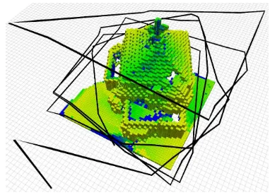
Figure 5. Result of the algorithm execution after 40 computed viewpoints. The black line represents the trajectory and the model in the center is the result of the reconstruction. The voxels
are colored according to their uncertainty.
a building at the University of Bonn called Frankenforst, whose 3D model stems from terrestrial laser scans of that building, see Figure 4. The exploration mission was specified using a bound-ing box with a size of29m×32m×25m. For the evaluation, we used 10 different runs defined through 10 sampled locations spaced on a circle on the ground around the building as starting locations for the MAV. At each location, the MAV started on the ground, performed a vertical take-off and then started the explo-ration mission using one of the three algorithms.
The camera has a field-of-view of 86◦and a resolution of 2040 by 2040 pixels, and was mounted on the front of the MAV facing downwards with an angle of 45◦, taking the images at a constant framerate of20 Hz. In order to realize a fair comparison (same resolution and sensing range), we set all the parameters for the al-gorithms to the default values provided by Isler et al. (2016), with the exception of the camera calibration, the ray caster resolution (reduced by a factor of 2), and the ray caster range of20m.
At each step of the next-best-view selection of our exploration algorithm, we recompute the bounding box as the hull of all non-free space cell, i.e. all cells that have never been observed or contain a measured point. Each time the new bounding box is recomputed, we sample 100 viewpoints as possible next view-points around it. For the comparison with Isler et al. (2016) and Vasquez-Gomez et al. (2014), we disabled our time-dependent cost function and introduced in the other two algorithms a bool-ean cost function to prevent collisions, as the implementation by Isler et al. (2016) does not provide a functioning collision avoid-ance system. We stopped the three algorithms after a fixed num-ber of viewpoints were approached.
Precision of the Reconstruction
First, we analyze the precision of the 3D reconstruction by con-sidering the uncertainties in the point estimates on the surface of the building. With these experiments, we show that each new viewpoint effectively reduces this uncertainty and increases the number of observed voxels and we compare our approach with two state-of-the-art methods.
0 5 10 15 20 25 30 35 40
Figure 6. Global uncertainty of the map at each viewpoint.
0 5 10 15 20 25 30 35 40
Figure 7. Total number of explored voxels in the map at each viewpoint.
al. (2016), which runs at100 Hzon a MAV and operates with an uncertainty of few centimeters.
Figure 5 illustrates an example of a computed trajectory around the building and the precision of the reconstructed 3D model us-ing a voxel resolution of0.5m. Each voxel is colored according to the total uncertainty of the points it contains, as described in the following color scheme:
• Blue to green: the points in this voxel have shown a high uncertainty.
• Green: Medium uncertainty.
• Green to yellow: 3D point estimates with small uncertainty. Further observation will not reduce the uncertainty of the point estimates substantially.
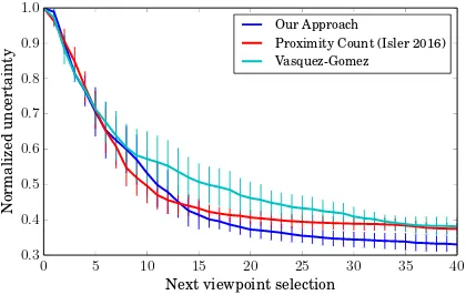
For a more quantitative evaluation, Figure 6 shows how the malized global uncertainty evolves during exploration. The nor-malized global uncertainty is equal to the global uncertainty di-vided by the maximum possible uncertainty. The maximum pos-sible uncertainty is easily computed by summing the uncertainty of every voxel before the exploration starts. In addition to that, Figure 7 also shows the total number of explored voxels in the map over time. As can be seen from these figures, the three algo-rithms show similar performances on both uncertainty reduction and voxel count, with a slight advantage of our approach.
Path Smoothness
A relevant aspect when planning a trajectory for a flying robot is the shape of the flight path. The reason for that is the need of a human supervisor to monitor any autonomous MAV at all times—this is required by law in several countries. From our experience, an important aspect for the path is to avoid abrupt
40 60 80 100 120 140 160 180
Figure 8. Cumulative histogram of the changes of motion direction.
Figure 9. Trajectory length at each viewpoint.
changes in the flight direction. This allows a human operator to understand more easily the robot’s path and intervene if needed. As Figure 5 shows, our approach can compute paths that are fairly regular and avoid zig-zag flight maneuvers. It basically performs larger turns if the model requires it.
To obtain a more quantitative measure and to compare the smoothness of each algorithm’s output trajectory, we analyzed the angle of every change of direction taken by the MAV. Figure 8 shows in histogram form the cumulative percentage of changes of direction for angles between40◦
and180◦
, divided in 10 inter-vals. As can be seen, our algorithm computed next-best-views that leads to smaller changes in the direction of flight, thanks to our utility function, which takes into account the angle of the new point w.r.t. the current direction of motion. In particular, the fig-ure shows how our algorithm avoids most of the time (about 80% of the cases) to choose a point at an angle above 100◦, while the other algorithms show a linear trend on the plot, i.e. it will be harder to predict how abrupt the next turn might be.
Path Length
0 100 200 300 400 500 600 700 Path length [m]
0 .3 0
.4 0.5 0
.6 0
.7 0
.8 0.9 1
.0
N
or
m
a
li
z
ed
u
n
cer
ta
in
ty
Our Approach
Proximity Count (Isler 2016) Vasquez-Gomez
Figure 10. Map uncertainty versus traveled distance.
0 200 400 600 800 1000 1200 1400
Time [s] 0
.3
0
.4
0
.5
0
.6
0
.7
0
.8
0
.9
1
.0
N
or
m
a
li
z
ed
u
n
cer
ta
in
ty
Our Approach
Proximity Count (Isler 2016) Vasquez-Gomez
Figure 11. Map uncertainty versus elapsed time.
Table 2. Average time and std. deviation to compute a viewpoint with the different algorithms.
Algorithm Average Time and std. deviation [s] Our algorithm 1.31 (±0.41)
Proximity Count (Isler 2016) 6.53 (±1.56) Vasquez-Gomez 6.58 (±1.56)
Execution Time
Additionally, we measured the execution time of the three ap-proaches. Table 2 shows the average time spent to compute the next viewpoint. It indicates an advantage of our approach in terms of execution time. In addition to that, Figure 11 shows the uncer-tainty against the elapsed time. As can be seen, our approach reduces the uncertainty faster while the time elapses.
Real World Experiment
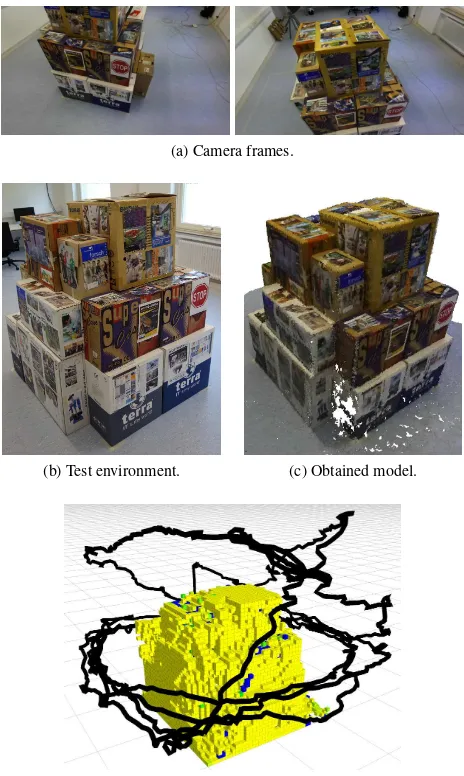
To test our algorithm outside the simulated environment, we cre-ated a structure of boxes in an indoor scene (Figure 12b). Fig-ure 12d shows the path of the stereo camera and the voxelized model obtained, with a resolution of0.05mper voxel side. Fig-ure 12a shows a couple of frames from the camera during the exploration procedure and Figure 12c shows the final 3D model that has been reconstructed from the recorded images. The dense model depicted in Figure 12c has a much higher resolution than the voxels of the octree and thus has been computed off-line us-ing an out-of-the-box Visual-SLAM approach. No contribution for the Visual-SLAM approach itself is claimed here.
Time-Dependent Cost Function
As the final aspect, we aim at illustrating the capability of our algorithm of guiding the MAV back to the starting point before the battery is empty. We achieve this using a time-dependent cost
(a) Camera frames.
(b) Test environment. (c) Obtained model.
(d) Voxel reconstruction and followed path.
Figure 12. Real world experiment.
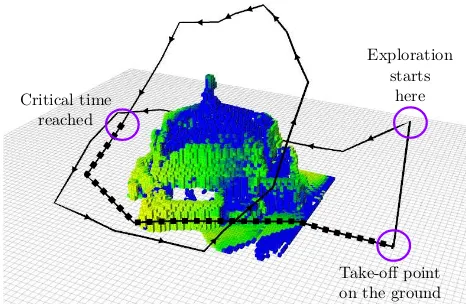
function that becomes active after a critical time (alternatively through monitoring the battery status). This critical time is com-puted dynamically according to the trajectory needed to reach the starting point from the current location. This cost function prefers locations that guide the MAV towards the starting point on com-parably safe paths, while still trying to reduce the uncertainty of the map. Figure 13 shows a path computed with a time limit. At first, the algorithm explores normally the building (black contin-uous path), but when the critical time is reached, as shown by the square markers, the MAV flies towards the starting point, while still trying to reduce the uncertainty, keeping a low altitude and avoiding to fly above obstacles.
CONCLUSIONS
Take-off point on the ground Critical time
reached
Exploration starts
here
Figure 13. Path computed with the time-dependent cost function enabled. The square markers represent the path generated after
the critical time, which moves the MAV back to the starting point.
experiments show that our approach allows for a precise recon-struction while flying on a comparably smooth trajectory without sacrificing the path length and performs well compared to exist-ing methods.
Despite these encouraging results, there is further space for im-provements. First and most important, we will provide real world experiments outdoors exploring a full building. Second, we plan to relax the assumption of equal uncertainty of each point in an image and thus taking into account the current image content.
ACKNOWLEDGEMENTS
This work has partly been supported by the DFG under the grant number FOR 1505: Mapping on Demand.
References
Aloimonos, J., Weiss, I. and Bandyopadhyay, A., 1988. Active vision.Intl. Journal of Computer Vision (IJCV)1(4), pp. 333– 356.
Atanasov, N., Le Ny, J., Daniilidis, K. and Pappas, G. J., 2015. Decentralized active information acquisition: theory and appli-cation to multi-robot slam. In:Proc. of the IEEE Intl. Conf. on Robotics & Automation (ICRA), pp. 4775–4782.
Bajcsy, R., 1988. Active perception. Proceedings of the IEEE 76(8), pp. 966–1005.
Bircher, A., Alexis, K., Burri, M., Oettershagen, P., Omari, S., Mantel, T. and Siegwart, R., 2015. Structural inspection path planning via iterative viewpoint resampling with application to aerial robotics. In:Proc. of the IEEE Intl. Conf. on Robotics & Automation (ICRA), pp. 6423–6430.
Charrow, B., Kahn, G., Patil, S., Liu, S., Goldberg, K., Abbeel, P., Michael, N. and Kumar, V., 2015. Information-theoretic planning with trajectory optimization for dense 3d mapping. In:Proc. of Robotics: Science and Systems (RSS).
Forster, C., Pizzoli, M. and Scaramuzza, D., 2014. Appearance-based active, monocular, dense reconstruction for micro aerial vehicle. In:Proc. of Robotics: Science and Systems (RSS).
Fraundorfer, F., Heng, L., Honegger, D., Lee, G. H., Meier, L., Tanskanen, P. and Pollefeys, M., 2012. Vision-based au-tonomous mapping and exploration using a quadrotor mav. In: Proc. of the IEEE/RSJ Int. Conf. on Intelligent Robots and Sys-tems (IROS), pp. 4557–4564.
Freundlich, C., Mordohai, P. and Zavlanos, M. M., 2013. A hybrid control approach to the next-best-view problem using stereo vision. In:Proc. of the IEEE Intl. Conf. on Robotics & Automation (ICRA), pp. 4493–4498.
Hornung, A., Wurm, K. M., Bennewitz, M., Stachniss, C. and Burgard, W., 2013. Octomap: an efficient probabilistic 3d mapping framework based on octrees. Autonomous Robots 34(3), pp. 189–206.
Isler, S., Sabzevari, R., Delmerico, J. and Scaramuzza, D., 2016. An information gain formulation for active volumetric 3d re-construction. In: Proc. of the IEEE Intl. Conf. on Robotics & Automation (ICRA), pp. 3477–3484.
Kriegel, S., Bodenm¨uller, T., Suppa, M. and Hirzinger, G., 2011. A surface-based next-best-view approach for automated 3d model completion of unknown objects. In:Proc. of the IEEE Intl. Conf. on Robotics & Automation (ICRA), pp. 4869–4874.
Mostegel, C., Wendel, A. and Bischof, H., 2014. Active monocu-lar localization: towards autonomous monocumonocu-lar exploration for multirotor mavs. In: Proc. of the IEEE Intl. Conf. on Robotics & Automation (ICRA), pp. 3848–3855.
Nieuwenhuisen, M. and Behnke, S., 2016. Layered mission and path planning for mav navigation with partial environment knowledge. In: Intelligent Autonomous Systems 13, Springer, pp. 307–319.
Perea Strom, D., Nenci, F. and Stachniss, C., 2015. Predic-tive exploration considering previously mapped environments. In: Proc. of the IEEE Intl. Conf. on Robotics & Automation (ICRA), pp. 2761–2766.
Pizzoli, M., Forster, C. and Scaramuzza, D., 2014. Remode: Probabilistic, monocular dense reconstruction in real time. In: Proc. of the IEEE Intl. Conf. on Robotics & Automation (ICRA), pp. 2609–2616.
Reinhardt, M., Noack, B. and Hanebeck, U. D., 2012. Closed-form optimization of covariance intersection for low-dimensional matrices. In:Proc. of the Int. Conf. on Informa-tion Fusion, pp. 1891–1896.
Sadat, S. A., Chutskoff, K., Jungic, D., Wawerla, J. and Vaughan, R., 2014. Feature-rich path planning for robust navigation of mavs with mono-slam. In: Proc. of the IEEE Intl. Conf. on Robotics & Automation (ICRA), pp. 3870–3875.
Schmid, K., Hirschm¨uller, H., D¨omel, A., Grixa, I., Suppa, M. and Hirzinger, G., 2012. View planning for multi-view stereo 3d reconstruction using an autonomous multicopter.Journal of Intelligent and Robotic Systems (JIRS)65(1-4), pp. 309–323.
Schneider, J., Elnig, C., Klingbeil, L., Kuhlmann, E., F¨orstner, W. and Stachniss, C., 2016. Fast and effective online pose estima-tion and mapping for uavs. In:Proc. of the IEEE Intl. Conf. on Robotics & Automation (ICRA).
Scott, W., Roth, G. and Rivest, J.-F., 2003. View planning for au-tomated 3d object reconstruction inspection.ACM Computing Surveys.
Stachniss, C., Grisetti, G. and Burgard, W., 2005. Information gain-based exploration using rao-blackwellized particle filters. In:Robotics: Science and Systems, pp. 65–72.
Strasdat, H., Stachniss, C. and Burgard, W., 2009. Which land-mark is useful? learning selection policies for navigation in unknown environments. In: Proc. of the IEEE Intl. Conf. on Robotics & Automation (ICRA), Kobe, Japan.
Vasquez-Gomez, J. I., Sucar, L. E., Murrieta-Cid, R. and Lopez-Damian, E., 2014. Volumetric next-best-view planning for 3d object reconstruction with positioning error. Intl. Journal of Advanced Robotic Systems.