Modelling technical change in Italian agriculture:
a latent variable approach
Roberto Esposti
a,∗, Pierpaolo Pierani
baDipartimento di Economia, Università di Ancona, Piazzale Martelli, 8, 60121 Ancona, Italy bDepartment of Economics, University of Siena, Siena, Italy
Received 28 October 1997; received in revised form 19 November 1999; accepted 28 December 1999
Abstract
This paper presents an alternative approach to the measurement of technical change. It is based on the latent variable level
of technology that enters explicitly the input demand system and on a hypothesis about the innovation generating process. By
adding measurement error equations, the behavioral system can be viewed as a Multiple Indicators/Multiple Causes (MIMIC) model. The parameter estimates are obtained with a maximum likelihood estimator which involves the implicit covariance matrix. The analysis refers to Italian agriculture and the results provide some evidence on the nature and level of technical change during the years 1961–1991. © 2000 Elsevier Science B.V. All rights reserved.
Keywords: Italian agriculture; MIMIC model; Total factor productivity (TFP); Technical change
1. Introduction
In this paper, we develop an econometric model to analyze the sources of growth of output and to esti-mate the rate of technical change in Italian agriculture for the period 1961–1991. Since World War II, agri-cultural output has risen at remarkable rates, labor has steadily diminished and capital has commonly been considered scarce. In other words, output growth can only be partly explained by changes in input use. One could therefore conclude that the agricultural sector in Italy registered sustained rates of technical progress, at least during the investigation period.
∗Corresponding author. Tel.:+39-071-2207119;
fax:+39-071-2207102.
E-mail address: [email protected] (R. Esposti)
Though, it is generally accepted that technological innovation influences output growth enhancing total factor productivity (TFP), conventional TFP indexes often give an inadequate account of the real contri-bution of technical change. Solow (1957) is usually cited as the seminal study in this field. Nonetheless, some aspects of his elegant accounting framework appeared open to criticism right from the beginning. The residual measure implicitly assumes that techni-cal change is exogenous which essentially amounts to leaving it unexplained. TFP growth can be viewed as the fundamental outcome of technical change but it cannot be identified with it. Not only can it be an erroneous measure of such change but, more funda-mentally, it does not provide any information about how technical change is generated. A great deal of literature has focused on the explanation of technical change, in particular, trying to introduce so-called
non-conventional inputs, such as R&D and Extension expenditure, human capital accumulation, spillover effects. Contributions can be divided into two big strands of literature. The first focuses on the theoreti-cal aspects. In a general economic equilibrium frame-work, the idea is to model why some agents invest time or money in R&D, human capital accumulation, etc. thereby fostering technical change. This is sub-stantially the approach of the so-called endogenous (or new) growth theory (Lucas, 1986; Jones, 1995).
A second research field is essentially empirical. It does not aim at explaining why technical change oc-curs; rather, it wants to provide empirical evidence of the link between technical change and its measured re-sult (TFP) and the non-conventional inputs mentioned above. Although it may seem less ambitious and based upon ad hoc assumptions, it has attracted much at-tention. This paper is a contribution to this strand of literature.
In applied work, the crucial point is that we can-not observe the real technological level, and, con-sequently, the estimation of the relation between non-conventional inputs and technological change becomes problematic. To tackle it, three strate-gies have been proposed. The first assumes that non-conventional inputs (most frequently R&D) are good proxies of technological level and therefore in-troduces them explicitly into the aggregate production function (or dual functions) together with conven-tional inputs. Many results for the agricultural sector have been presented (Huffman and Evenson, 1989; Khatri and Thirtle, 1996; Mullen et al., 1996; Kuroda, 1997) also for the case of Italy (Esposti and Pierani, 1999). However, results using this approach are only reliable to the extent that non-conventional variables are good proxies of the underlying technological level. A second approach is based upon the so-called TFP decomposition and it implies two stages.1 In the first, TFP growth calculation is carried out, with technical change being approximated by the time trend. The pro-ductivity index is then regressed on non-conventional inputs to estimate their impact and contribution to technical change. Many results have also been pro-duced for the agricultural sector using this approach (Thirtle and Bottomley, 1989; Evenson and Pray, 1991;
1It is also called two-stage approach while the first one-stage or integrated approach.
Fernandez-Cornejo and Shumway, 1997; Alston et al., 1998a) including for the Italian case (Esposti, 1999). However, if TFP growth is a poor proxy of real techni-cal change, this approach runs into econometric prob-lems, due to the inconsistency of parameter estimates caused by measurement errors (Fuller, 1987).
A third alternative has recently been suggested (Gao, 1994; Gao and Reynolds, 1994). It uses the con-cept of technology as a latent variable. Both TFP and non-conventional inputs can be regarded as proxies but they measure it with errors that can greatly affect estimates, and this also partially explains why such different results can be found in the literature (Alston et al., 1998b). Moreover, while TFP is the observed effect of technical change, non-conventional inputs are observed possible causes of it. Latent variable models can handle these issues well: technological level explicitly enters the production process, while the economic process generating it and involving non-conventional inputs is formally specified. This structure can be represented in a unified analytic form and simultaneously estimated in the so-called Multiple Indicators/Multiple Causes (MIMIC) model. This paper applies this latent variable approach to Italian agriculture. The main aim is to stress the dif-ferences that can emerge with respect to alternative methods. Moreover, some emphasis is also put on data sources and the construction of variables, as we think, these are crucial aspects that can highly affect latent variable estimates and explain the above-mentioned differences.
2. MIMIC model specification
Long run agricultural production in Italy is depicted from the dual by means of the differential approach (Theil, 1980). It consists of one aggregate output (q), four inputs (materials (xM), labor (xL), capital (xK), land (xT)) and the unobservable technology level (4).2 The derived input demand function can be viewed as first-order Taylor series approximation to a
general demand system and takes the form (Barnett, 1979; Gao and Reynolds, 1994):3
sid(logxi)= X
k
µikd(logpk)+ωθid(logq)
+βid(log4), i=1, . . . ,4 (1)
where: si is the i-th cost share; d (log) represents a logarithmic change of relevant variables; ω is the cost flexibility;4 θi indicates the i-th marginal cost share; µik is the Slutsky coefficient; βi=siτi, and
τi=∂(log xi)/∂(log4) is the technology elasticity of the i-th input. Technological change is defined to be input i-using, -saving or -neutral depending on whether βi is positive, negative or nil, respectively. On the other hand, overall neutrality implies that
βi=0 for all i.
Since4 is not observable, it is not possible to es-timate directly from Eq. (1) with standard regression tools. We have to turn to latent variable econometrics. Following Jöreskog and Sörbom (1989), we indicate with η=(η1,η2,. . .,ηm) a latent vector of endoge-nous variables describing the state of agriculture and with ξ=(ξ1,ξ2,. . .,ξn) a vector of exogenous vari-ables which have an influence on the state. Formally, each period relationship between the two vectors can be expressed by the following system of linear
struc-tural equations:
η=Bη+Ŵξ+ζ (2)
where, B (m×m) andŴ(m×n) are matrices of
coeffi-cients andς=(ς1,ς2,. . .,ςm) denotes a typical dis-turbance vector. It is assumed that ς and ξ are not correlated and the matrix (I–B) is nonsingular. By def-inition, the latent vector, usually only some element in it, is not observable. Instead, we can observe an indi-cator y=(y1, y2,. . ., yp) which is related toηthrough measurement equations, such that:
y =3yη+ε (3)
3The augmented Dickey–Fuller test is performed to test the sta-tionarity. The results indicate that all variables used in the anal-ysis are nonstationary since we cannot reject the null hypothesis of unit root. Assuming trend-stationary processes, the differential approach seems a sensible solution to avoid spurious results and inconsistent estimates (Plosser and Schwert, 1978; Granger and Newbold, 1981; Clark and Youngblood, 1992).
4We setω=1, as this is the value consistent with an aggregate cost function (Chambers, 1988).
where,3y(p×m) is a matrix of parameters. The error termεis assumed not to be correlated withς andη, but there can be correlation within systems.
The equation system Eqs. (2) and (3) is often re-ferred to as MIMIC model in that it may contain mul-tiple indicators and mulmul-tiple causes of the unobserved variables. In this study, technological progress is con-ceptualized as taking place in two separable stages: generating innovations potentially available to agri-culture; selecting innovations and determining a mea-surable outcome, namely, productivity growth. The exogenous vector represents the generation and the in-troduction of innovations into the agricultural sector. The state vector describes the process in which the op-timal combination of inputs is determined, conditional on the level of technology, output and factor prices.
The rational for assuming4 exogenous has to do with one of the main features of agriculture in Italy, namely, the prevalence of small farms and price-taker behavior. Incapable of their own innovative strategies farmers adopt rather than produce innovations. An important issue is the specification of the influences thought to affect the technological level but beyond the control of farmers. A number of exogenous shifters are considered including public R&D and Extension ex-penditures, human capital, and international and inter-sectoral spillover. Though in applied work, the choice of these cause variables and methods of construction are still subject to debate, there is widespread recog-nition that knowledge capital approximated by public R&D and Extension variables is pivotal. Being quan-titatively negligible, private research does not play a relevant role and it is not considered.5 When innova-tions are made available to properly informed farm-ers, the extent and speed of their adoption depend on the skill and innovative attitude of the farmers. The human capital variable synthesizes this capability. In fact, agricultural innovations mostly originate from outside the sector, at least in Italy. The importance of intersectoral and international spillovers of technol-ogy have been well emphasized in literature (Bouchet et al., 1989) and demonstrated for Italian agriculture (Esposti, 1999). Accordingly, we have modelled the innovation process with the following exogenous
gen-erating function:
4=Sg(R, I, H ) (4)
where S is the international and intersectoral technol-ogy spillover.6 R and I indicate public agricultural
research and extension services, respectively, and H, human capital. All explanatory variables in Eq. (4) are treated as predetermined stocks. This equation is sim-ply a descriptive device motivated by heuristic argu-ments. Log differentiating Eq. (4) with respect to time yields:
˙
4= ˙S+εRR˙+εII˙+εHH˙ (5)
where4˙ =∂ln4/∂t,εR=∂ln g(.)/∂ln R, and so on. In addition, if we are willing to assume that the ratio of the potential spillover to the whole new interna-tional and intersectoral technological knowledge7 is constant(γT = ˙S/T )˙ , then:
˙
4=γTT˙+γRR˙+γII˙+γHH˙ (6)
Combining the demand system Eq. (1) with Eq. (6), we get the latent variable model to be estimated. Structural equations can be represented as follows:
6We separate explicitly this variable in the expression of the technology generation function as it is a prerequisite to have innovative opportunities at sectoral level.
7As also indicated in Khatri and Thirtle (1996), not all new technological and scientific knowledge is potentially relevant for agriculture. S expresses this potential as a constant share of the entire production of new knowledge represented by the T variable.
The parameter restrictions implied by symmetry (µik=µki), homogeneity of degree 0 of the demand functions P
kµik =0,∀i
and adding-up of the sys-tem P
iβi,Piµik=0,∀k,Piθi =1
are imposed in estimation (Selvanathan, 1989). In our case, the land share equation is omitted and the remaining three in-put demands are expressed in terms of relative prices, with land as numeraire.8
All cause variables in Eq. (6) are observable. How-ever, the presence of unobserved technical change requires measurement equations. Through them, we represent the latent variable with the growth rate of TFP explicitly taking into account the error with which the indicator measures the unobserved variable (Aigner and Deistler, 1989).
In our model, the system of measurement equations takes the form:
where, ε1 denotes a typical disturbance term. The MIMIC model (Eq. (7)–(8)) is a special case of Lin-ear Structural Model with Latent Variables (LISREL) for the presence of only one endogenous latent vector (Jöreskog and Goldberger, 1975; Bollen, 1989). The parameters are estimated using LISREL 7.2 software with a maximum likelihood procedure.9
8 Indirect estimates of the other parameters in the omitted land share equation can be obtained rearranging the restrictions of the demand system in terms of the directly estimated parameters as follows: βT=−(βM+βL+βK), µMT=−(µMM+µML+µMK), µLT=−(µML+µLL+µLK), µKT=−(µMK+µLK+µKK), µT T=
3. Data sources and methods of construction
Annual time series for conventional inputs and out-put have been obtained as Fisher indexes of relevant prices and quantities from the AGRIFIT database of Italian agriculture which is described more fully in Caiumi et al. (1995). Agricultural output aggregates 52 products, but it does not comprise self produced inputs while it includes deficiency payments and other pro-duction subsidies. Four conventional inputs are consid-ered in the analysis: intermediate consumption, labor, land and capital. The latter put together three broad categories: machinery and durable equipment, non-residential structures and livestock. Labor consists of self employed farmers and hired workers. Intermediate consumption includes purchased feeds, fertilizer, pes-ticides, seed, energy, repair and maintenance, etc. The TFP index comes from Pierani and Rizzi (1994).10
We next look at the way the exogenous influences are specified in the generating function in Eq. (6). Among the causes that may influence the unobserved technological level, we have considered public R&D and Extension expenditures, human capital, and inter-national and intersectoral spillover. These are briefly discussed in turn.
The intersectoral and international technological stock (T) is captured by the number of domestic and foreign patent demands in United States. The extent to which this data can act as a good indicator of technological advance is often criticized. However, with Griliches (1994), we argue that the number of annual patent demands is the result of both recent R&D investment and cumulated knowledge stock. In other words, we consider it a good proxy of all technological knowledge. The spillover variable (S) represents the percentage of T which can potentially benefit agricultural productivity; hence, we expect that 0< γT <1.
The substitution of US patents for international knowledge capital is common practice. In their study of UK agriculture, Khatri and Thirtle (1996) justify adopting them because they seem to perform better in
10This measure explicitly accounts for quasi-fixity of some fac-tors, namely, family labor and capital. The authors use a General-ized Leontief form (Morrison, 1992). Their restricted cost function consists of one aggregate output three variable inputs, two quasi fixed factors and time trend.
term of explanatory power than EU patents. However, they consider only patents for agricultural chemi-cals and machinery. In Italy, there is some evidence that patented innovations useful for agriculture orig-inate from different sectors and technological fields (Esposti, 1999) so we consider all patents and let the data determine the percentage actually relevant for agriculture.11 Instead, Fernandez-Cornejo and Shumway (1997) have chosen US agricultural TFP as proxy for international knowledge capital. This vari-able might turn out to be a poor alternative when the study concerns agricultural sectors whose structures are markedly different from US agriculture as is the case of Italy.
An important issue which arises when using patent data is that values change over time as consequence of economic growth and cycle. Empirically, their mar-ket valuations are not observed, hence we adjusted US patent data for the long-run OECD-countries pro capite GDP growth (Griliches, 1994).
Public R&D and Extension (R and I variables) ex-penditures are obtained from Italian Ministry of Agri-culture and Forestry, public local extension services and the accounts of other relevant Institutions. A list of specific sources, and a detailed explanation of the data and construction of the variables used in this study can be found in Esposti (1999). The data refers to research funding by the Ministry of Agriculture and Forestry, and expenditure by both specialized public research institutes and public University Faculties of Agricul-ture and Animal Science. ExpendiAgricul-ture is expressed in billions of 1985 Italian lire.
To convert time series of R&D and Extension ex-penditures into stocks we follow the perpetual in-ventory method as slightly modified by Park (1995). The stock of research (similarly for extension) accu-mulates according to the following expression:Rt =
ItR−mR+(1−δ
R)R
t−1, whereItRis gross investments. A number of alternatives exist regarding either the length or the shape of the lag profiles. Unfortunately, with few exceptions (Nadiri and Prucha, 1993), the assumptions underlying this conventional procedure
have not been statistically tested. Typically, one has to assume more or less arbitrary values for both the ini-tial gestation lag (m), before investments become ef-fective, and the (constant) rate of depreciation (δ). We setδR=0.1, mR=4 (Park, 1995; Kuroda, 1997). Given that Extension programs have faster and shorter-lived impacts than R&D (Evenson and Westphal, 1995), we setδI=0.3 and mI=3.
Finally, concerning human capital (H), we proxy it with farmers education. Following analogous studies (Gao and Reynolds, 1994), we measure farmers edu-cation by their average years of schooling.
Given the assumed parameters, the final sample ranged from 1961 to 1991.
4. Empirical results and discussion
The results of estimation of model (Eq. (7)–(8)) are presented in Table 1. The upper part of the table sets out estimates of the input demand system. The empir-ical evidence seems to reject the hypothesis of Hicks neutrality, to support the evidence of labor-using tech-nical change, and to be inconclusive with respect to materials and capital whose coefficients are not statis-tically significant. This picture is something of a nov-elty if compared to the application of an analogous methodology to US agriculture (Gao and Reynolds, 1994) and to other approaches applied to the Italian case (Pierani and Rizzi, 1991) where labour saving and capital and materials using biases are frequently registered.
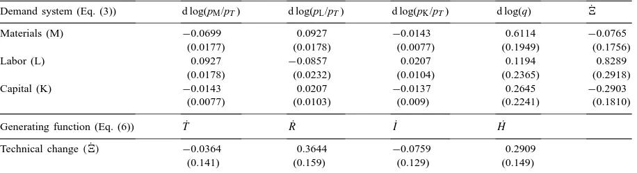
Table 1
Parameter estimates of the MIMIC model (standard errors in parenthesis)a
Demand system (Eq. (3)) d log(pM/pT) d log(pL/pT) d log(pK/pT) d log(q) 4˙
Materials (M) −0.0699 0.0927 −0.0143 0.6114 −0.0765
(0.0177) (0.0178) (0.0077) (0.1949) (0.1756)
Labor (L) 0.0927 −0.0857 0.0207 0.1194 0.8289
(0.0178) (0.0232) (0.0104) (0.2365) (0.2918)
Capital (K) −0.0143 0.0207 −0.0137 0.2645 −0.2903
(0.0077) (0.0103) (0.009) (0.2241) (0.1810)
Generating function (Eq. (6)) T˙ R˙ I˙ H˙
Technical change(4)˙ −0.0364 0.3644 −0.0759 0.2909
(0.141) (0.159) (0.129) (0.149)
aVariance of ε
1=0.0004, (0.0001); squared multiple correlation of TFP=0.335; coefficient of determination of structural equations=0.8422.
On one hand, we can think the differences are real. Indeed, Italian and US agriculture present deep struc-tural differences. In Italy, very small family farms are predominant and excess of labor, and capital and land scarcity are the norm. What we observe then is a bias consistent with these structural constraints, which al-low labor to be retained within the sector by raising its productivity relative to the other factors. This pattern looks quite original, although there is no economic reason to think that agriculture should inevitably move toward capital intensification. An increase of capital intensity is indeed observed but it is mainly due to rel-ative prices rather than technological change. If this is so, however, our results contrast with the induced innovation hypothesis.
On the other hand, this real explanation still leaves the question open as to why different results are ob-tained for Italian agriculture using different method-ologies and model formulation. In particular, the ways of representing technical change appear to be crucial. Usually, the technological level it is approximated by a time trend, while here the trend variable does not play any role as the technological change is entirely determined by the dynamics of non-conventional in-puts, that can drive and also invert technological bi-ases. Consequently, the choice of the data and the con-struction of the variables are crucial and can greatly affect results. In particular, the definition of R&D and Extension stocks is a well-known open question in the literature (Alston et al., 1998a).
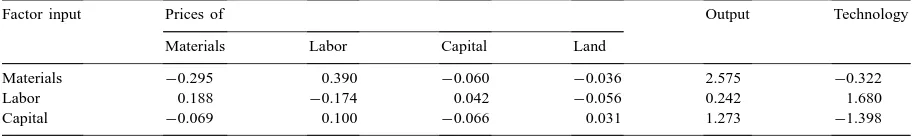
selec-Table 2
Price, output and technology elasticities14
Factor input Prices of Output Technology
Materials Labor Capital Land
Materials −0.295 0.390 −0.060 −0.036 2.575 −0.322
Labor 0.188 −0.174 0.042 −0.056 0.242 1.680
Capital −0.069 0.100 −0.066 0.031 1.273 −1.398
tion and definition of non-conventional inputs can be critical. According to the estimated parameters, exten-sion (I) and technological spillover (T) growths turn out to be not statistically significant while research (R) and human capital (H) have positive and significant impacts. Gao and Reynolds (1994) found similar re-sults. The null impact of I can be explained by the dif-ficulty in separating Extension and R&D effects due to their high collinearity (Mullen et al., 1996). The result of T suggests that a more detailed and precise definition of intersectoral and international technolog-ical spillover is needed; in fact, the present estimate indicates that this variable is not well approximated by a simple constant share of total US patents. R is the most relevant and significant variable in determining a labor-using technical change. We can interpret this result as the consequence of a conscious political be-havior to direct public agricultural research programs towards labor-intensive techniques and products. Al-ternatively, it could also be that an inappropriate def-inition of the R&D stock determines such an unusual labor-using bias.
Other information on agricultural technology can be obtained looking at the estimated price and output coefficients in Table 1 and at the compensated elastic-ities in Table 2.12 Most of the price coefficients are statistically significant and the own-price effects on the main diagonal are correctly signed with the excep-tion of land. Unfortunately, it is not possible to check whether the land price is statistically relevant as an es-timate of its standard error is missing. Cross-price co-efficients suggest complementarity between materials and capital, whereas, labor is a substitute for both ma-terials and capital. Therefore, the known dichotomy between an intensive use of capital and materials and
12Elasticities are calculated at the normalization point of data.
that of labor emerges. In this respect, our results con-firm previous analyzes (Pierani and Rizzi, 1991).
Price responses are quite unelastic and smaller than output and technology elasticities. As a consequence, long-run factor demands are only partially determined by relative price changes. For instance, with respect to labor, the technical change elasticity is the highest while output and relative prices have smaller impacts. In fact, labor share has been constantly decreasing during the estimation period in favor of materials and capital. Such a transformation is entirely due to the in-crease of the relative price for labor, as technological bias works in the opposite direction. These contrast-ing effects resulted in a progressive reduction of the number of agricultural workers.
At the footnote of Table 1, we report some statistical indicators of the model (Bollen, 1989; Jöreskog and Sörbom, 1989). First of all, the estimate of the vari-ance of the error termε1turns out to be significantly different from zero. This result shows that we cannot substitute the latent variable with the indicator vari-able without introducing a bias due to measurement errors (Fuller, 1987). In other words, introducing TFP measure in the demand system would eventually give inconsistent estimates. The squared multiple
correla-tion and the total coefficient of determinacorrela-tion give an
idea of the performance of each component block: the former refers to measurement Eq. (8), the latter to the structural Eq. (7). It turns out that the variation of TFP seems to be a poor proxy of the unobservable tech-nical change. Nonetheless, it remains the best proxy available. After all, it is just the awareness of the in-adequacy of our proxies that makes the latent variable model a sensible alternative.
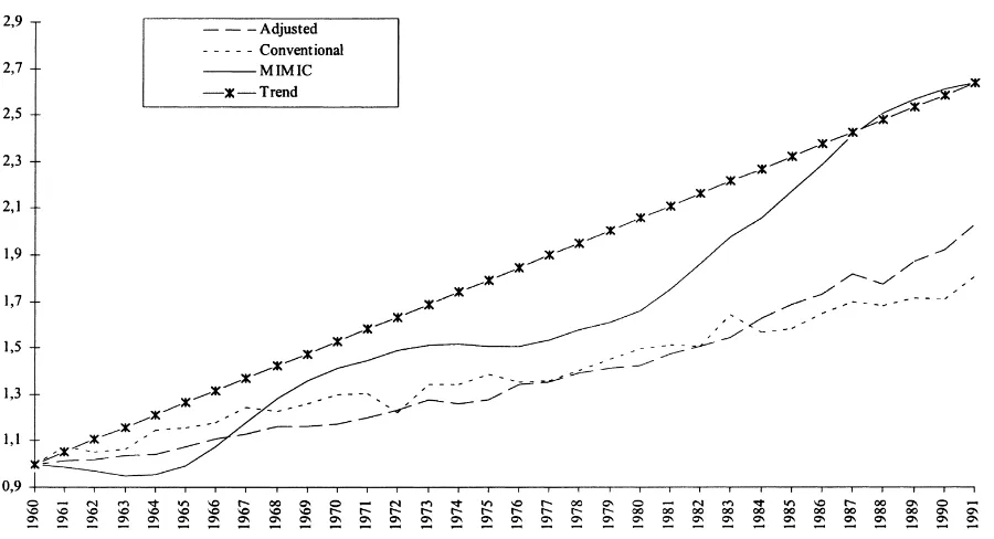
Fig. 1. Technology indexes over time.
Table 3
Technological change indexes (computed at the period means) Period MIMIC4˙ Conventional TFP Adjusted TFP
1961–1991 0.031 0.019 0.023
1961–1971 0.034 0.024 0.017
1972–1981 0.014 0.015 0.021
1982–1991 0.043 0.016 0.029
the quasi-fixity of some input13 (Pierani and Rizzi, 1994). The profiles of the three indices are drawn in Fig. 1, whereas, sub-period averages are reported in Table 3. The MIMIC estimate of technical change shows differences with respect to the TFP measures. In the MIMIC case, the average rate of growth over the whole period is 3.1%; this measure is higher than the conventional and the adjusted ones, 1.9 and 2.3%, respectively. According to our model, therefore, full-and/or sub-equilibrium TFP growth measures tend to underestimate technical progress.
Looking at the subperiod averages, the MIMIC re-sults seem to show a sort of medium-term cyclical
13This is the variable actually used as indicator of technical change in the MIMIC model.
behavior: fast growth in the 60’s, a remarkable slow down during the seventies and the highest rates in the eighties. Considering Fig. 1, one can see that the MIMIC measure shows a more regular path, too (Gao and Reynolds, 1994). This feature is due to the ex-plicit presence of measurement errors, so that the latent variable estimation can take into account variations in the indicator variables that are not related to technol-ogy (particularly in agriculture, short-run factors like weather and other shocks can affect TFP measure-ment). This smoothness can also allow MIMIC mea-sure to detect long or medium term cyclical patterns of agricultural technical change better. Therefore, the latent variable approach seems to be recommendable whenever the interest focuses on long run behavior rather than short run response.
5. Summary and concluding remarks
growth. Theoretically, the two concepts are linked, as higher productivity is the final outcome of a technical advance, but they cannot be confused as is the case in the traditional approach. Technical change is a plex economic and institutional process and its com-prehension is at least as important as its measurement. The MIMIC representation turns out to be useful in both respects: representing the generation process and measuring technical change. The model provides consistent estimates of the structural parameters and is flexible enough to allow potentially for a dynamic specification of the generating process. However, this alternative has not been explored in this study.
The empirical results provide some evidence of the positive impact of public R&D expenditure on the technological level in agriculture and also the increase of human capital expressed by education level seems significant. These variables play a relevant role in the structural transformation of the sector. As it is labor-using, technical change partially compensates for the tendency to substitute labor with capital and materials due to their relatively lower prices.
The MIMIC measure of technical change turns out to be different both from the conventional and ad-justed TFP measures that appear to underestimate such change. Their profiles over time are also quite differ-ent. The MIMIC results reveal a cyclical behavior in the medium-long run along with a particularly intense technological growth in the 80’s, probably caused by the declining of traditional and inefficient agricultural systems.
The latent variable approach can outperform tradi-tional approaches also providing empirical informa-tion about the causes of technical change. However, even the MIMIC model requires TFP measures as proxies. On the other hand, TFP measures are still relatively easier and less computationally expensive. Essentially, the choice between the alternative ap-proaches depends on the objective of the research project.
Acknowledgements
The authors are listed alphabetically, and authorship can be attributed as follows: introduction and Sections 2 and 4 to Pierani, Sections 1 and 3 to Esposti. They wish to thank J.P. Chavas, P.L. Rizzi and an
anony-mous referee for their helpful comments on an earlier version. Of course, responsibility for views expressed and remaining errors is their own.
References
Alston, J.M., Craig, B., Pardey, P., 1998a. Dynamics in the creation and depreciation of knowledge and the returns to research, EPTD Discussion Paper 35. IFPRI, Washington, DC. Alston, J.M., Marra, M.C., Pardey, P.G., Wyatt, T.J., 1998b.
Research returns redux: a meta-analysis of the returns to agricultural R&D, EPTD Discussion Paper 38. IFPRI, Washington, DC.
Aigner, D.J., Deistler, M. (Eds.), 1989. Latent variable models. Annal. J. Econ. 41.
Barnett, W.A., 1979. Theoretical foundations for the Rotterdam model. Rev. Econ. Studies. 50, 109–130.
Bollen, K.A., 1989. Structural Equations with Latent Variables. Wiley, New York.
Bouchet, F.C., Orden, D., Norton, G.W., 1989. Sources of growth in French agriculture. Am. J. Agric. Econ. 71, 281–293. Caiumi, A., Pierani, P., Rizzi, P.L., Rossi, N., 1995. AGRIFIT: una
banca dati del settore agricolo (1951–1991). Franco Angeli, Milano.
Chambers, R.G., 1988. Applied Production Analysis. Cambridge University Press, Cambridge.
Clark, J.S., Youngblood, C.E., 1992. Estimating duality models with biased technical change: a time series approach. Am. J. Agric. Econ. 74, 353–360.
Esposti, R., 1999. Spillover tecnologici e progresso tecnico agricolo in Italia. Rivista di Politica Economica 90, in press. Esposti, R., Pierani, P., 1999. Investimento in R&S e produttività
nell’agricoltura italiana (1963–91): un approccio econometrico mediante una funzione di costo variabile. In: L’agricoltura italiana alle soglie del XXI secolo. Proceedings of the XXXV Meeting of Italian Agricultural Economists, 10–12 September 1998, Palermo, in press.
Evenson, R., Pray, C.E. (Eds.), 1991. Research and Productivity in Asian Agriculture. Cornell University Press, Ithaca, NY. Evenson, R.E., Westphal, L.E., 1995. Technology change and
technology strategy. In: Behrman, J., Srinivasan, T.N. (Eds.), Handbook of Development Economics, Vol. 3. Elsevier, Amsterdam.
Fernandez-Cornejo, J., Shumway, C.R., 1997. Research and productivity in Mexican agriculture. Am. J. Agric. Econ. 79, 738–753.
Fuller, W., 1987. Measurement Error Models. Wiley, New York. Gao, X.M., 1994. Measuring technical change using a latent
variable approach. Eur. Rev. Agric. Econ. 21, 13–119. Gao, X.M., Reynolds, A., 1994. A structural equation approach to
measuring technological change: an application to southeastern US agriculture. J. Prod. Anal. 5, 123–139.
Granger, C.W., Newbold, J., 1981. Spurious regression in econometrics. J. Econ. 55, 121–130.
Huffman, W.E., Evenson, R.E., 1989. Supply and demand functions for multiproduct US cash grains farms: biases caused by research and other policies. Am. J. Agric. Econ. 71, 761– 773.
Jones, C.I., 1995. R&D-based models of economic growth. J. Polit. Econ. 103, 759–784.
Jöreskog, K.G., Goldberger, A.S., 1975. Estimation of a model with multiple indicators and multiple causes of a single latent variable. J. Am. Statist. Assoc. 70, 631–639.
Jöreskog, K.G., Sörbom, D., 1989. LISREL 7: User’s Reference Guide. Scientific Software Inc., Mooresville, USA.
Khatri, Y., Thirtle, C., 1996. Supply and demand functions in UK agriculture: biases of technical change and the returns to public R&D. J. Agric. Econ. 47, 338–354.
Kuroda, Y., 1997. Research and extension expenditures and productivity in Japanese agriculture, 1960–1990. Agric. Econ. 16 (2), 111–124.
Lucas, R.E., 1986. On the Mechanics of Economic Development. Queen’s Institute for Economic Research Discussion Paper 657. Mullen, J.D., Morrison, C.J., Strappazzon, L., 1996. Modelling technical change in Australian broadacre agriculture using a translog cost model. Paper presented at the Georgia Productivity Workshop II, University of Georgia, November 1–3. Morrison, C.J., 1992. A micreconomic approach to the
measurement of economic performance. Springer, New York.
Nadiri, M.I., Prucha, I.R., 1993. Estimation of the depreciation rate of physical and R&D capital in the US total manufacturing sector. NBER WP 4591, Washington, DC.
Park, W.G., 1995. International R&D spillovers and OECD economic growth. Econ. Inquiry 33, 571–591.
Pierani, P., Rizzi, P.L., 1991. Produttività totale dei fattori e progresso tecnico nell’agricoltura italiana: Un confronto Nord-Sud. Quaderni del Dipartimento di Economia Politica 130, Siena.
Pierani, P., Rizzi, P.L., 1994. Equilibrio di breve periodo, utilizzazione della capacità e produttività totale dei fattori nell’agricoltura Italiana (1952–1991). UREA Discussion Paper 13, Dipartimento di Economia Politica, Siena.
Plosser, C.I., Schwert, G.W., 1978. Money, income and sunspots: Measuring economic relationships and the effects of differencing. J. Monetary Econ. 4, 637–660.
Selvanathan, E.A., 1989. Advertising and consumer demand: a differential approach. Econ. Lett. 31, 215–219.
Solow, R.M., 1957. Technical change and the aggregate production function. Rev. Econ. Statist. 39, 312–320.
Thirtle, C., Bottomley, P., 1989. The rate of return to public sector agricultural R&D in the UK, 1965–80. Appl. Econ. 21, 1063– 1086.