Estimating sensible and latent heat flux densities from
grapevine canopies using surface renewal
D. Spano
a,∗, R.L. Snyder
b, P. Duce
c, K.T. Paw U
b aUniversita’ della Basilicata, Dip. di Produzione Vegetale, Facolta’ di Agraria, I-85100 Potenza, ItalybUniversity of California, Atmospheric Science, Davis, CA 95616, USA cConsiglio Nazionale delle Ricerche, IMAes, I-07100 Sassari, Italy Received 26 October 1999; received in revised form 23 May 2000; accepted 7 June 2000
Abstract
Fine-wire thermocouples were used to measure high-frequency temperature above and within canopies and structure functions were employed to determine temperature ramp characteristics, which were used in a fundamental conservation of energy equation to estimate sensible heat flux density. Earlier experiments over dense, tall, and short canopies demonstrated that the surface renewal method works, but requires a correction for uneven heating (e.g.α=0.5 for tall, andα=1.0 for short canopies). For sparse canopies, theαcalibration factor was unknown. Experiments were conducted in grape vineyards in California and Italy to determine whether the surface renewal method works in a sparse canopy and to determine if calibration is necessary. Surface renewal data were collected at several heights in the canopies and these were compared with simultaneous 1-D sonic anemometer measurements. The results indicated that the surface renewal technique provides good estimates of sensible heat flux density under all stability conditions without the need for calibration when the data are measured at about 90% of the canopy height. The values were generally within ca. 45 W m−2of what was measured with a sonic anemometer. Separating the canopy into two layers provided even more accurate estimates of sensible heat flux density without the need for calibration. The best results were obtained when the lower layer was below the bottom of the vegetation and the upper layer included the vegetation. When combined with energy balance measurements of net radiation and soil heat flux density, using a thermocouple and the surface renewal technique offers an inexpensive alternative for estimating evapotranspiration with good accuracy. © 2000 Elsevier Science B.V. All rights reserved.
Keywords: Energy balance; Eddy-covariance; Temperature ramps; Coherent structures
1. Introduction
Energy balance measurements over full canopies are common; however, little information is avail-able on the energy balance over sparse grapevine canopies. Grape vineyards consist of widely spaced
∗Corresponding author. Tel.:+39-079-229336;
fax:+39-097-229337.
E-mail address: [email protected] (D. Spano).
plants that allow for deep penetration of sunlight and air turbulence into the canopy. As a result, the soil contribution to the energy balance is considerable. Because the radiative energy balance at the bottom of the canopy is greater than in canopies that are more closed, management of the vineyard floor can have a major effect on sensible (H) and latent (λE) heat flux density. This makes estimating crop evapo-transpiration more complicated than for more dense canopies. Therefore, it is desirable to have a robust
method for measuring crop evapotranspiration in situ.
Several researchers have investigated the determi-nation of evapotranspiration (λE) of grapevines using energy balance. Ham et al. (1991) and Ham and Heil-man (1991) used a sap flow heat balance technique to measure the transpiration of vines and a Bowen ratio system to estimateλE in a grape vineyard to separate crop evapotranspiration into transpiration and soil evaporation components. Oliver and Sene (1992) used eddy-covariance to measure λE over grapevines and they concluded that soil and vines are independent energy systems with little interaction between them. However, Heilman et al. (1994) showed that sensible heat from the exposed soil surface is a major contrib-utor to the canopy energy balance and transpiration of the vines. They concluded that the soil and the canopy are not independent and that the soil energy balance does affect energy balance of the vines. In a later study Heilman et al. (1996) showed that the canopy architecture has a substantial effect on soil and canopy energy balance, mainly by changing the partitioning of vineyard net radiation into its soil and canopy components. Trambouze et al. (1998) used eddy-covariance to measureλE from vineyards. They reported good λE estimates with very small time scale information, but they recommended against us-ing eddy-covariance for estimatus-ing actual evapotran-spiration of a vineyard because of the maintenance requirements. Because equipment for the Bowen ra-tio and eddy-covariance methods is expensive and requires a fairly high level of expertise to operate, a less expensive and more robust method is desirable for determining evapotranspiration of agricultural crops.
Tillman (1972) first reported the use of high-frequency temperature variance data to estimate H. He obtained good results during unstable atmospheric conditions when the data were corrected for stabil-ity. Later, Weaver (1990) used temperature variance data, similarity theory, and calibration coefficients that vary depending on the surface and energy bal-ance to determine H over semi-arid grass and brush. When corrected for stability, Lloyd et al. (1991) and De Bruin et al. (1993) also observed good estimates of H using temperature-variance data collected over sparse, dry land vegetation, stones, pebbles, etc. In all of these experiments, the method worked only
under unstable conditions, and a stability parameter was needed for the calculations. Paw U et al. (1995) studied the use of the variance method during stable conditions and reported that it was inaccurate for data taken within a meter or two of the canopy height for a maize crop, a walnut orchard, and a mixed deciduous forest. Clearly, the temperature variance method has little utility for measuring H over canopies with high evaporation rates that are likely to have near neutral atmospheric conditions close to the surface. Also, a temperature-based method that requires complicated measurements for determining a stability parameter has little practical value. In recent years, the surface renewal (SR) method has shown promise to provide estimates of H from high-frequency temperature data regardless of and without a measure of stability con-ditions.
The objective of this study was to evaluate: (1) the SR method for estimating H in grape vineyards; (2) the possibility of estimating H without the a factor (α=1.0) by separating the canopy volume into layers; and (3) the accuracy of the SR method for determining
λE as a residual term of the energy balance.
2. Theory
The SR method is based on the idea that traces of high-frequency temperature data above and within plant canopies exhibit ramp-like shapes that are re-lated to coherent structures (Paw U and Brunet, 1991). The mean ramp characteristics include the amplitude
a, and inverse ramp frequency, l+s, where l is the ramp
duration and s the time between ramps. During a mea-surement interval, the ramp characteristics are used in SR analysis to estimate H using a fundamental energy conservation equation (Paw U et al., 1995; Snyder et al., 1996; Spano et al., 1997b). The use of H esti-mated from SR analysis in conjunction with measured net radiation Rnand soil heat flux density G can
pro-vide an easily transportable and relatively inexpensive method to estimateλE.
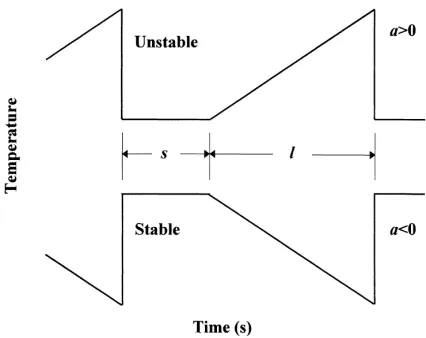
Fig. 1. Schematic temperature ramps with amplitude a>0 for un-stable and α<0 for stable atmospheric conditions. The inverse ramp frequency l+s in seconds is the sum of the quiescent period s and the ramp duration l.
et al., 1992). When the atmospheric conditions are unstable, warm air ejects from the canopy and cold air sweeps in to replace it. Then the temperature trace shows a sharp decrease followed by a slow increase until the next sweep and ejection (Fig. 1). The dura-tion of a ramp l is the length of time during which the air parcel is being heated. In addition, there is a quiescent period of time of duration s between ramp events. The quiescent period occurs during the transi-tion time when the cold air parcel ejects from and the warm air parcel sweeps into the canopy. The mean temperature amplitude and the length of time l+s for
a mean ramp during a sample interval determines the rate of heat transfer (Snyder et al., 1996; Spano et al., 1997b).
The rate at which air parcels heat or cool is related to the sensible heat flux between the canopy and the air above. Assuming uniform heating of an air volume
V, the change in heat content1C is expressed as a
function of the change in temperature with time (dT/dt) as
1C=ρCpdT
dt V (1)
whereρ is the air density and Cpthe specific heat of
air at constant pressure. If the change is measured over a surface with area A, H is calculated as
H=α1
whereα1is added to account for uneven heating within the air volume and z is the height of the air volume (measurement height). Because temperature data are measured at a fixed point, one must relate this ‘local’ change of temperature with time (in one dimension) to the total time derivative of temperature:
dT
Substituting for dT/dt in Eq. (2) and rearranging terms,
H can be expressed as a linear function
H=β+αρCp ∂T
∂t z (4)
whereβ represents a micro-scale advection term, and
αincludes effects of uneven temporal heat distribution in the canopy air and advective effects (Paw U et al., 1995). Paw U and Brunet (1991) tested this equation and reported that in the absence of advection,∂T/∂x≈0 andβ≈0. Therefore,
H≈αρCp ∂T
∂t z (5)
When high-frequency temperature data are mea-sured and analyzed for average ramp characteristics, the change in temperature per unit time (∂T/∂t) — as
the temperature increases or decreases during a ramp — is equal to the amplitude divided by the length a/l; so, for the sensible heat transfer during the ramps, one obtains
Hr=αρCpa
lz (6)
During the quiescent period, there is no apparent change in temperature with time (and no sensible heat flux), so Hris multiplied by the relative time for
heating l/(l+s) to account for the total time of ramp
activity and quiescent periods. Therefore, Eq. (7) provides an estimate of the sensible heat flux density during the sampling period:
the temperature is measured at the canopy top, there is uneven heating and α<1.0. For example, Paw U et al. (1995) found α≈0.5 for temperature data col-lected at the canopy top of a forest, walnut orchard, and maize crop. However, dT/dt was determined us-ing low pass filterus-ing, and not structure functions. For short canopies, when the temperature was collected above the canopy top, theαvalues were variable, but closer to 1.0 (Snyder et al., 1996; Spano et al., 1997b). Differences in results were attributed to more even heating above a canopy than within a canopy and a different methodology to estimate dT/dt. In all cases, theαfactor was determined by empirical calibration against sonic anemometer measurements.
In early research, smoothing techniques were used to eliminate the independent random turbulent part of the scalar signal, leaving only the coherent organized part (Paw U et al., 1995; Katul et al., 1996), which is used in SR analysis to determine ramp characteris-tics. However, a simpler method for calculating a and
l+s involved the use of a structure function and
sta-tistical moments as suggested by Van Atta (1977). A simple explanation of the procedure was presented in the Appendix of Snyder et al. (1996). This approach gave good results over several crops (Snyder et al., 1996; Spano et al., 1997b; Anandakumar, 1999). Chen et al. (1997) presented a modified structure function approach to estimate H, assuming a sloping rather than a vertical temperature change at the end of a ramp. This eliminates the quiescent period s between ramps. Using this approach, they found good results for data collected over straw mulch, forest, and bare soil.
In previous experiments, the plant canopies studied were variable in height, but all had dense foliage. In a sparse canopy (e.g. grape vineyard), the ground is only partially covered, and less differential heating of the air volume below the measurement height is expected than in a forest, walnut orchard, or maize crop, which were reported to have α≈0.5 (Paw U et al., 1995). When data were collected at heights well above the top of short canopies with α≈1.0, there was a con-siderable volume of air under the measurement height when there was no vegetation. In a sparse vineyard, there is less vegetation than the tall, dense canopies and more vegetation than for the short canopies, so 0.5<α<1.0 was expected in the vineyards with data from the canopy top.
3. Materials and methods
Three experiments were conducted to test the use of the SR method in measuring energy balance in grape (Vitis vinifera L.) vineyards. The first experi-ment was conducted in 1995 in the Oakville Field Sta-tion in Napa Valley, CA (latitude 38◦26′N; longitude 122◦24′W; elevation 58 m above m.s.l.). The Cabernet Sauvignon grapevines were oriented in north–south rows with 1.2 m between plants and 2.7 m between rows, they were about 2.0 m tall, and there was≈100 m of fetch in the upwind direction (south) during the experiment. The canopy was estimated to have about 65% ground cover. The vines were irrigated with a drip irrigation system and trained in a conventional curtain system. High-frequency (f=8 Hz) temperature data were collected at the canopy top (2.0 m) and at 2.3, 2.6, and 2.9 m, using single-wire 76-mm diame-ter thermocouples. Net radiation (3.5 m height), soil heat flux density (0.02 m depth), sensible heat flux density (3.0 m height), and latent heat flux density (3.0 m height) were measured using a net radiome-ter (model Q-7, REBS, Seattle, WA), three soil heat flux plates (REBS, Seattle, WA), a sonic anemometer (model CA27. Campbell Scientific, Logan, UT), and a krypton hygrometer (model KH20, Campbell Scien-tific, Logan, UT).
A second experiment was conducted in 1996 in a grape vineyard near Villasor, Italy (latitude 39◦24′N; longitude 8◦54′W; elevation 22 m above m.s.l.). The vines were ≈10-year-old Pinot bianco tops on 1103 Paulsen rootstock. There was a curtain training system with 1.2 m between plants and 2.7 m between rows. The rows were oriented east–west and the vines were irrigated with drip irrigation. The height of the canopy was 2.1 m and there was an ≈200 m fetch. Again, ground cover was about 65%. Temperature data were collected below and above the canopy at heights of 1.5, 1.8, 2.1, 2.4 and 2.7 m with 76-mm diameter ther-mocouples. Energy balance sensors were the same as those used in California.
The fetch was >200 m with a canopy ground cover of
≈65%. The vineyard was flood-irrigated during the season, but not during the experiment. High-frequency (f=8 Hz) temperature data were collected at the canopy top (2.2 m) and at 0.3 m intervals below the canopy height (1.0, 1.3, 1.6, and 1.9 m). A 1-D eddy-covariance system (CA27 sonic anemometer and KH20 krypton hygrometer) was mounted at 2.5 m above the ground, and net radiation (Rn) was
mea-sured at the 3-m height. Six heat flux plates were installed at the 0.08-m depth and two thermocouples were buried at depths of 0.02 and 0.06 m near each of the plates to determine the soil heat flux density
G. The G data were collected from a transect
start-ing at the middle of one row and at 0.5 m intervals in the direction of an adjacent row that was 3.0 m west. A 3-D sonic anemometer (Campbell Scientific CSAT3) was also used in this experiment, but unfor-tunately was only working when the surface renewal thermocouples were not operational. However, both the 1-D and this 3-D sonic anemometers did provide some coincidental data with a root mean square error (Me) equal to 24 W m−2, providing confidence in the accuracy of the 1-D sonic data.
In all three experimental vineyards, the foliage was evenly distributed within the upper two-thirds of the canopy height. The foliage was dense within that vol-ume, but the canopy covered only about 65% of the horizontal surface area, so about 35% of the soil was exposed to the sky.
All temperature data were collected using a Campbell Scientific CR10 data-logger. The sample lags for calculating the structure functions were j=2, 4, 6, and 8 corresponding to time lags of r=0.25, 0.50, 0.75, and 1.00 s. Following the approach of Van Atta (1977), the second, third, and fifth powers of a structure function were used to estimate a and l+s. A
detailed description of calculations can be found in the Appendix to Snyder et al. (1996):
Sn(r)= 1
where m is the number of data points in the time in-terval, j a sample lag between data points correspond-ing to a time lag (r=j/f), and Ti the ith temperature sample in the interval. One assumption in using the structure function of Van Atta (1977) is that the time
lag r is much smaller than l+s. Therefore, the
result-ing values of l+s were screened for a minimum value
of 5r s, with maximum value of 900 s. When l+s<5r, then H was considered to be missing data. This oc-curred rarely during day time. When l+s>900 s, then H was set equal to zero.
High-frequency temperature data from each mea-surement height were used to determine SR estimate of H (HS) using the volume of air from the soil surface
to the measurement height. Sensible heat flux density was also calculated layer-wise within the canopy us-ing temperature measurements at the top of each layer and assuming uniform heating within the layer below the measurement height (α=1.0). If heating of the air volume below a measurement height is uniform, then temperature fluctuations measured at the top provide ramp characteristics that represent the entire layer, and they can be used to estimate the uniform change in transient heat content of the underlying layer. If heat-ing is not vertically uniform, then calculatheat-ing ramp characteristics at several heights allows for the deter-mination of transient sensible heat content changes ac-cording to the layer, assumingα=1.0 for each layer. This is true because, as the vertical thickness of an air volume decreases, heating within an air layer be-comes more uniform andαapproaches 1.0. Summing the change in heat content over all layers gives the change in heat content of the full air volume under the highest measurement. Because the ejection of air from the canopy involves the transfer of the entire vol-ume of air under the highest measurement, separating the air volume into layers provides a method to more accurately estimate total sensible heat flux density HS
without calibrating forα. In the Villasor experiment, the H values were summed over two layers (0–1.5 and 1.5–2.1 m) to determine HS. In the Satiety experiment, HS was determined for two different combinations of two layers. The first set of two layers was 0–1.3 and 1.3–2.2 m. The second set of two layers was 0–1.0 and 1.0–2.2 m.
In all cases, the SR method H values (HS) were
compared with H values from a 1-D sonic anemome-ter (HE). Corrections for uneven heatingαwere
cal-culated using a regression of HE versus HS through
HE. Calculations of the mean HS were also done
us-ing four time lags (r=0.25, 0.50, 0.75, and 1.00 s) and compared with HE.
Estimates of latent heat flux density as a residual term of the energy budget were calculated using HS
(λES) and HE (λEE) along with the same Rn and G
values. BothλEEandλESvalues were compared with λE values from an eddy-covariance system (λEK). The
WPL correction (Webb et al., 1980) was applied to the eddy-covariance data forλE.
As it is a measure of both bias and variance from the 1:1 line, the root mean squared error Me statistic was used to compare HS with HE, and λES andλEE
High-frequency temperature data collected at the canopy top were used to calculate the Tillman (1972) variance method for estimating H under unstable, free convection conditions using
where C1=0.95 is a universal constant (Tillman,
1972), k the von Karman constant (k=0.41), g the acceleration due to gravity (0.98 m s−2),σ
T the
stan-dard deviation of the temperature, and T¯ the mean temperature during the sampling interval. Informa-tion on stability type was evaluated from measured
HE values. Comparisons between HE and HT were
done only when HE was positive and the wind speed
was<2.0 m s−1, so that the assumed free convection conditions leading to Eq. (10) were likely to be met.
Table 1
Weighting factor α, coefficient of determination R2, root mean square error Me, and number of half-hour samples for HEvs. HS
measurements taken over 2.0-m tall grapevines at the Oakville Field Station in Napa Valley, CA on 14–15 August 1995a Height (m) α R2 Me(W m−2) n
2.0 0.88 0.80 44 33
2.3 0.81 0.74 62 34
2.6 0.76 0.76 76 34
2.9 0.66 0.81 111 34
aRegressions were forced through the origin and the M
e is
between HSand HE. HSwas calculated using the mean of the 0.25 and 0.50-s time lags. The range of HE was−45 to –326 W m−2.
4. Results and discussion
4.1. Comparison according to measurement height
The mean HS of the r=0.25 and 0.50 s time-lag
calculations compared with HE values are shown in
Table 1 for the Napa Valley experiment. Table 1 also gives the correction for unequal heatingα, coefficient of determination R2, root mean square error Me, and number of half-hour period n. The largest value for
α and the lowest Me were observed at the canopy top (2 m). The α values decreased and the Me in-creased with measurement height above the canopy. The canopy topα values of 0.88 were considerably higher than theα=0.5 value reported for forest, wal-nut, and maize canopies (Paw U et al., 1995), butαwas
<1.0 for grass (Snyder et al., 1996) and for wheat and sorghum (Spano et al., 1997b). Similar results were obtained using the mean of the r=0.25, 0.50, 0.75, 1.00 s time lags.
The results from the experiment at Villasor are shown in Table 2 for the mean HSfrom the r=0.25 and
0.50 s time lags. Again, the smallest Mewas found for data taken at the canopy height (2.1 m). Theαvalue (0.89) for the canopy top (2.1 m) was nearly the same as found in the Napa Valley experiment. Both within and above canopy α values decreased with height. Assuming a linear change inα with height between 1.8 and 2.1 m,α=1.0 is expected at 1.85 m (88% of the canopy height) for the data from Table 2. As found in the Napa Valley data, using the mean of r=0.25, 0.50, 0.75 and 1.00 s time lags gave similar results.
Table 2
Weighting factor α, coefficient of determination R2, root mean square error Me, and number of half-hour samples for HE vs. HS
measurements taken over 2.1 m tall grapevines at Villasor, Italy on 23–26 July 1996a
Height (m) α R2 Me (W m−2) n
1.5 1.31 0.84 58 88
1.8 1.02 0.88 33 96
2.1 0.89 0.93 34 97
2.4 0.75 0.77 71 61
2.7 0.77 0.91 60 94
aRegressions were forced through the origin and the M
e is
between HSand HE. HSwas calculated using the mean of the 0.25 and 0.50-s time lags. The range of HE was−25 to –329 W m−2.
shown in Table 3 for the mean HS from the r=0.25
and 0.50 s time lags. Again, the smallest Mewas found for the measurements taken at the canopy height. The
α=0.74 value for the canopy top was slightly smaller than the values found in Napa Valley and Villasor. However, the height where α=1.0, based on the as-sumption of a linear trend from 1.9 to 2.2 m, was about
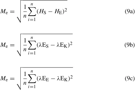
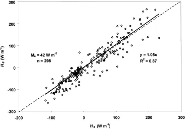
Fig. 2. Eddy-covariance HE vs. mean surface renewal HS sensible heat flux density using the time lags r=0.25 and 0.50 s from data collected at Villasor during 23–26 July 1996. HSwas determined as the sum of two layers where the layers were from z=0 to 1.5 m and from z=1.5 to 2.1 m. The solid line represents a linear regression forced through the origin and the dashed line the 1:1 line.
Table 3
Weighting factor α, coefficient of determination R2, root mean square error Me, and number of half-hour samples for HEvs. HS
measurements taken over 2.2-m tall grapevines at Satiety Vineyard, Woodland, CA on 11–20 September 1998a
Height (m) α R2 Me(W m−2) n
1.0 2.93 0.59 61 305
1.3 1.68 0.50 57 318
1.6 1.37 0.58 51 344
1.9 1.09 0.81 42 397
2.2 0.74 0.86 54 434
aRegressions were forced through the origin and the M
e is
between HSand HE. HSwas calculated using the mean of the 0.25 and 0.50-s time lags. The range of HE was−162 to –265 W m−2.
1.98 m (90% of the canopy height) for the Table 3 data. The results were relatively independent of time lag, similar to the previous experiments.
is heated or cooled evenly and other factors are neg-ligible,α=1.0 is expected. In all experiments, the HS values overestimated H at and above the canopy top measurements (α <1) and underestimated H at heights below the canopy top (α>1). In both cases, a decrease in α with height was obtained. This was consistent with the theory discussed by Paw U et al. (1995) and the results reported in previous experiments (Spano et al., 1997a, b). Theαvalues depend on the temper-ature measurement level in relation to the postulated height to which the renewal volume was heated or cooled during the ramp event.
When the measurement level is higher than the mean height of the air volume being heated or cooled, entrainment with air aloft could affect the estimation, and HSvalues result in an overestimate (α<1). When
the measurement level is lower than the mean height of the air volume being heated or cooled, air above the measurement level within the renewal parcel air is actually heated or cooled, but not accounted for in the energy balance in the parcel being considered. Thus,
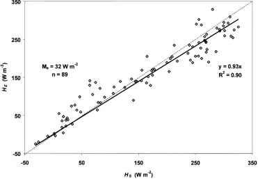
Fig. 3. Eddy-covariance HE vs. mean surface renewal HS sensible heat flux density using the time lags r=0.25 and 0.50 s from data collected at Satiety during 11–20 September 1998. HSwas determined as the sum of two layers where the layers were from z=0 to 1.3 m and from z=1.3 to 2.2 m. The solid line represents a linear regression forced through the origin and the dashed line the 1:1 line.
HS values result in an underestimate of H andαwill
be >1.
Based on the results of all the experiments, HS
val-ues from temperature data collected at about 90% of the canopy height would likely provide good estimates of H withα=1.0 (i.e. no calibration would be needed). It is expected that most of the results would be within about 45 W m−2of HE. There was little difference
ob-served between HS values coming from the mean of
two time lags or four time lags, so using 76-mm di-ameter thermocouples, the 8-Hz data, and time lags
r=0.25 and 0.50 s yield acceptable performance.
4.2. Layer-wise comparisons
Although good estimates of H from HS were
pos-sible without accounting for uneven heating of the air volume below the canopy top, a method to determine
HS without calibrating against HE is desirable. One
heating and cooling of the canopy air is related to the distribution of plant elements, temperature fluctua-tions could be uneven with height. Vertical variation in the heating can be sampled by sensors at two or more heights. Therefore, the SR heat flux can be cal-culated separately for each layer using fluctuation data from each height, which defines the top of each layer assuming uniform heating andα=1.0. The total heat flux from a canopy would equal the sum of the layer calculations. Thus, calculating the heat flux separately by layer and summing over layers should provide an estimate of H without the need for calibration to de-termineαfor the canopy. For practical purposes, the fewer the number of thermocouples needed the better. Therefore, the canopy was separated into two layers. The lower layer was from the ground to one height within the canopy, and the upper layer was from that level to the canopy top. Using the Villasor data, the layers were from z=0–1.5 m and from z=1.5–2.1 m. Most of the canopy foliage fell within the upper layer.
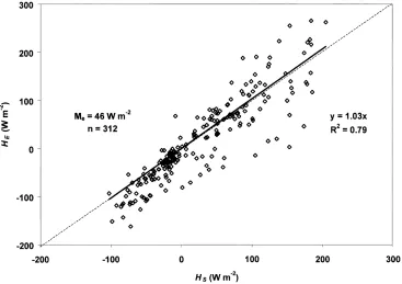
Fig. 4. Eddy-covariance HE vs. mean surface renewal HS sensible heat flux density using the time lags r=0.25 and 0.50 s from data collected at Satiety during 11–20 September 1998. HSwas determined as the sum of two layers where the layers were from z=0 to 1.0 m and from z=1.0 to 2.2 m. The solid line represents a linear regression forced through the origin and the dashed line the 1:1 line.
Fig. 2 shows the results when HSwas calculated as
the sum of H from the two layers. The layer H values were calculated as the mean H using the time lags
r=0.25 and 0.50 s. When compared with HE, there
was an improvement both in terms ofα and the Me over using only the canopy top data (Table 2).
A second test for using layers to eliminate the need for α was completed using the Satiety data. Fig. 3 shows the results when HS was calculated using the
sum of H estimates from the two layers z=0–1.3 m and z=1.3–2.2 m, which roughly correspond to the heights used in Villasor. Again, the layer H values were calculated as the mean H usingα=1.0 and time lags r=0.25 and 0.50 s. Theαvalue was considerably closer to unity and the Me was improved by using the layer estimates rather than using only the canopy top estimate of HS(Table 3). Although the z=1.3 m height
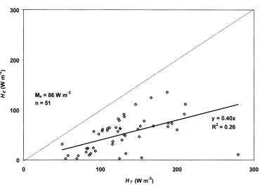
Fig. 5. Sensible heat flux density from eddy-covariance HEvs. the Tillman equation HT using data from Satiety during 12–15 September 1998.
the upper layer. When HS was calculated as the sum
of the two-layer H values using the time lags r=0.25 and 0.50 s, the Me was further improved (Fig. 4). Therefore, the best estimates of HS, without
calibrat-ing forα, were obtained using one layer below the fo-liage and the other layer including most of the fofo-liage. Most likely, the air volume below the foliage had uni-form heating and the upper layer, containing the fo-liage, had uniform heating that was different from the lower layer. When determined separately and summed, the HS estimate was improved upon treatment of the
canopy as one layer.
4.3. Comparison with the variance method
Using data from Satiety, estimates of sensible heat flux density (HT) using the Tillman (1972) equation
were calculated and compared to H (Fig. 5). Be-cause there was insufficient data to determine the Monin–Obukhov stability function (L), only the free convection equation of Tillman was used. Free con-vection is most likely to occur under unstable, low
wind-speed conditions. Therefore, we only used HT
values when HE was positive and when the wind
speed was<2.0 m s−1. The 2.0 m s−1value could be
too high for free convection conditions, but there were few data with lower wind speeds. Based on the results in Fig. 5, the variance method has limited utility for measuring over irrigated crops with highλE.
4.4. Energy balance calculations
When testing the SR method, HS is compared with HE estimates from a 1-D sonic anemometer. It was assumed that the HE values were accurate, but the
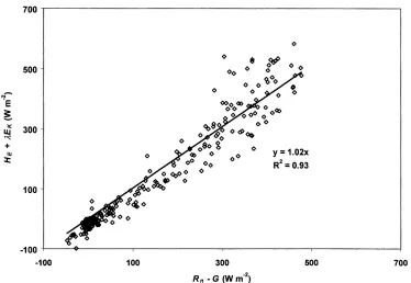
output was tested using energy balance closure. Fig. 6 is a plot of HE+λEKfrom a 1-D sonic anemometer and
a krypton hygrometer versus Rn−G for data from the
Satiety experiment. The slope was close to unity and the value of R2 was high, indicating a good closure. Therefore, it is likely that the 1-D sonic was providing accurate estimates of HE.
evapotranspi-Fig. 6. Sensible plus latent heat flux densities from eddy-covariance HE+λEK vs. net radiation minus soil heat flux density Rn−G from
Satiety during September 1998.
ration (λE) from grape vineyards using the energy balance equationλE=Rn−G−H. Comparison ofλES
andλEE values withλEK is shown in Table 4 for the
Satiety experiment.λES was calculated as the
resid-ual term of the energy budget using HS determined
as the sum of two layers. The results showed a slope
Table 4
Slope of the regression b, coefficient of determination R2, root mean squared error Me, and number of half-hour samples forλES
andλEEvs.λEK measurements taken over 2.2-m tall grapevines at Satiety Vineyard, Woodland, CA on 11–20 September 1998a
R2 M
e (W m−2) n
λEE 0.97 0.82 56 279 λES 0.94 0.78 58 297
aRegressions were forced through the origin and the M
e is
between λEE and λES and λES and λEK. λEE and λES were calculated as the residual terms of the energy budget using HE and HS, respectively. HSwas determined as the sum of two layers where the layers were from z=0 to 1.0 m and from z=1.0 to 2.2 m. The range ofλEK was−33 to−455 W m−2.
of the regression through the origin close to unity for
λEEand more scatter forλES. However, the Mevalue forλE, estimated as a residual of the energy budget, is approximately the same for surface renewal and eddy covariance. Based on the results from Satiety and assuming an accurate determination of Rnand G
(Fig. 6), the use of surface renewal H values, calcu-lated by layers, in an energy balance equation provides estimates ofλE within about 12% of values calculated using a sonic anemometer and a krypton hygrometer.
5. Conclusions
High-frequency (8 Hz) temperature data were col-lected at several heights within and above grape vineyards using 76-mm diameter thermocouples. The data were used to estimate sensible heat flux density
HSusing the surface renewal method. The ramp
lags gave nearly the same results. Therefore, using four time lags was unnecessary.
Earlier experiments over dense, tall canopies indi-cated that a calibration factor (α=0.5) was needed to adjust for uneven heating of the air volume when data were collected at the canopy top. Over dense, short canopies, anα=1.0 value was observed when the data were collected well above the canopy top. With the sparse grapevine canopies,αwas expected to be somewhere between 0.5 and 1.0. This research showed that theαvalues decreased with measurement height to <1.0 at the canopy top. Based on linear inter-polation, α≈1.0 was expected at about 90% of the canopy height. Therefore, future measurements at that level should provide H estimates with less than about 45 W m−2 error, without the need for α calibration. In contrast, based on this data set, the free convection Tillman (1972) method would not be recommended.
Calculating H separately for two layers in the canopy and summing to estimate HS withαfixed at
unity provided even better results with the maximum error expected to be between 32 and 42 W m−2. So summing over layers eliminated the need to empir-ically determine α. The best results were obtained when the lower layer was below the bottom of the foliage.
In conclusion, the surface renewal method, without calibration, offers a simple, relatively low cost method to estimate H over sparse grapevine canopies. When used in an energy balance equation, the method pro-vides good estimates ofλE for grapevines.
Acknowledgements
Partial support for this research was provided by the National Research Council (Italy) (NITCAR Project No. 115.06638.98.03286.ST74). This work was par-tially funded by the University of Sassari — 1998 Sci-entific Research 60% grant. A portion of this work was supported by grants to K.T. Paw U from the U.S. Department of Energy (DOE) National Institute for Global Environmental Change (NIGEC) through the NIGEC Western Regional Center at the University of California Davis (DOE Cooperative Agreement No. DE-FCO3-90ER61010). Any opinions, findings and conclusions or recommendations expressed herein are those of the authors and do not necessarily reflect the
view of the DOE. The authors wish to thank Dr. Ster-ling Chaykin for supporting the research at Satiety Vineyard and Winery in California and the Consorzio Interprovinciale per la Frutticoltura (Cagliari, Italy) for supporting research at Villasor in Italy. The authors thank the editor and the two anonymous reviewers for their helpful comments and suggestions.
References
Anandakumar, K., 1999. Sensible heat flux over a wheat canopy: optical scintillometer measurements and surface renewal analysis estimations. Agric. For. Meteorol. 96, 145–156. Chen, W., Novak, M.D., Black, T.A., 1997. Coherent eddies and
temperature structure functions for three contrasting surfaces. Part II: Renewal model for sensible heat flux. Boundary Layer Meteorol. 84, 125–147.
De Bruin, H.A.R., Kohsiek, W., Vandenhurk, B.J.J.M., 1993. A verification of some method to determine the fluxes of momentum, sensible heat and water vapor using standard deviation and structure parameters of scalar meteorological quantities. Boundary Layer Meteorol. 63, 231–257.
Gao, W., Shaw, R.H., Paw U, K.T., 1989. Observations of organized structure in turbulent flow within and above a forest canopy. Boundary Layer Meteorol. 47, 349–377.
Ham, J.M., Heilman, J.L., Lascano, R.J., 1991. Soil and canopy energy balances of a row crop at partial cover. Agron. J. 83, 744–753.
Ham, J.M., Heilman, J.L., 1991. Aerodynamic and surface resistances affecting energy transport in a sparse crop. Agric. For. Meteorol. 53, 267–284.
Heilman, J.L., McInnes, K.J., Savage, M.J., Gesch, R.W., Lascano, R.J., 1994. Soil and canopy energy balances in a west Texas vineyard. Agric. For. Meteorol. 71, 99–114.
Heilman, J.L., McInnes, K.J., Gesch, R.W., Lascano, R.J., Savage, M.J., 1996. Effects of trellising on the energy balance of a vineyard. Agric. For. Meteorol. 81, 79–93.
Katul, G., Hsieh, C., Oren, R., Ellsworth, D., Phillips, N., 1996. Latent and sensible heat flux predictions from a uniform pine forest using surface renewal and flux variance methods. Boundary Layer Meteorol. 80, 249–282.
Lloyd, C.R., Culf, A.D., Dolman, A.J., Gash, J.H.C., 1991. Estimates of sensible heat flux from observations of temperature fluctuations. Boundary Layer Meteorol. 47, 311–322. Oliver, H.R., Sene, K.J., 1992. Energy and water balances of
developing vines. Agric. For. Meteorol. 61, 167–185. Paw U, K.T., Brunet, Y., 1991. A surface renewal measure of
sensible heat flux density. Proceedings of the 20th Conference on Agriculture and Forest Meteorology, Salt Lake City, pp. 52–53.
Paw U, K.T., Qiu, J., Su, H.B., Watanabe, T., Brunet, Y., 1995. Surface renewal analysis: a new method to obtain scalar fluxes without velocity data. Agric. For. Meteorol. 74, 119–137. Snyder, R.L., Spano, D., Paw U, K.T., 1996. Surface renewal
analysis for sensible and latent heat flux density. Boundary Layer Meteorol. 77, 249–266.
Spano, D., Duce, P., Snyder, R.L., Paw U, K.T., 1997a. Surface renewal estimates of evapotranspiration. Tall canopies. Acta Hort. 449, 63–68.
Spano, D., Snyder, R.L., Duce, P., Paw U, K.T., 1997b. Surface renewal analysis for sensible heat flux density using structure functions. Agric. For. Meteorol. 86, 259–271.
Tillman, J.E., 1972. The indirect determination of stability, heat and momentum fluxes in the atmospheric boundary layer from
simple scalar variables during dry unstable conditions. J. Appl. Meteorol. 11, 783–792.
Trambouze, W., Bertuzzi, P., Voltz, M., 1998. Comparison of methods for estimating actual evapotranspiration in a row-cropped vineyard. Agric. For. Meteorol. 91, 193–208. Van Atta, C.W., 1977. Effect of coherent structures on structure
functions of temperature in the atmospheric boundary layer. Arch. Mech. 29, 161–171.
Weaver, H.L., 1990. Temperature and humidity flux-variance relations determined by one-dimensional eddy correlation. Boundary Layer Meteorol. 53, 77–91.