A method of land evaluation including year to year weather variability
Gordon Hudson
∗, Richard V. Birnie
Land Use Science Group, Macaulay Land Use Research Institute, Craigiebuckler, Aberdeen AB15 8HQ, Scotland, UK
Received 14 May 1999; received in revised form 5 November 1999; accepted 16 November 1999
Abstract
Land evaluation is sensitive to the effects of annual variability in weather. A method to incorporate this variability into land evaluation systems is proposed, using the land capability system for Scotland as a case study. Land capability classes were found to be sensitive to the climate reference period from which data are taken. Individual stations rarely occupy their long-term land capability class. In addition, the relative position of stations in the land classification alters from year to year, indicating variations with time in spatial correlation structures. Markov chain analysis was used in a risk assessment approach to estimate the mean return time to a land capability category for individual stations and for areas of land. The main conclusions were: that land evaluation systems should not be applied using data from a different period to the baseline weather period used to establish the classification; there is a need to establish whether groups of stations tend to behave in similar ways over space and through time; mapping zones of risk could provide a means of formally incorporating weather variability into land evaluation. ©2000 Elsevier Science B.V. All rights reserved.
Keywords: Land evaluation; Climate variability; Markov-chain; Risk assessment; Agriculture
1. Introduction
Land evaluation is internationally recognised for providing qualitative information about land, such as its cropping potential or land degradation risk. It comprises a range of methods developed to enable the assessment of land in terms of either capability for general land uses (e.g. agriculture, forestry) or suitability for specific crop types (e.g. wheat, bar-ley). Pioneering work on developing land evaluation systems was carried out in America (Klingebiel and Montgomery, 1961) and developed subsequently by the Food and Agricultural Organisation (FAO, 1984) for application mainly in Africa. In general, the
sys-∗Corresponding author. Tel.:+44-01224-318611;
fax:+44-01224-311556.
E-mail address: [email protected] (G. Hudson).
tems use a range of land qualities, derived from measurable land characteristics, to classify land. The land qualities are modelled values that include crop growth requirements (e.g. temperature regime, mois-ture availability), impinge on management practices (e.g. land workability) and affect land conservation (e.g. erosion hazard) (FAO, 1984). The land quali-ties are derived in a variety of ways. The simplest method is by direct conversion; e.g. the potential for mechanisation based on slope calculated from elevation differences. Indirect interpretation is made using relationships between land characteristics, e.g. soil hydraulic conductivity can be modelled from more easily measured soil properties such as texture or structure. Crop simulation models can be used to integrate several land qualities to predict yields.
There are several generic issues associated with the application of land evaluation. In particular, land
ities derived from measurements of dynamic variables (e.g. temperature) are converted to static variables for the purposes of land evaluation. For example, tem-perature measurements are converted to land qualities such as length of growing period or accumulated temperature summed over a growing period. These land qualities, derived for a single seasonal cycle, are then summarised over a sequence of consecutive years, generally using robust statistics (e.g. median). Long-term summaries are used to construct empirical land evaluation systems, exemplified by Bibby et al. (1982) and the FAO (1996). A key weakness in using summarised land qualities is that by treating dynamic variables in a static way much of the variability that is an essential property of the land is removed. Farmers do not farm average landscapes under average cli-matic conditions. So, whilst land evaluation methods based on this approach are of value in land use plan-ning, for land management decision making it may be more useful to have information on variability from which risk may be assessed.
There are few examples of land evaluation where dynamic variables have been explicitly included. van Lanen et al. (1992) showed that it is possible to de-velop a mixed approach for incorporating weather variability. In their method, land is first classified qual-itatively using biophysical or socio-economic data to form land evaluation units. Then dynamic variables are re-incorporated uniformly within each land evalu-ation unit using a representative climate stevalu-ation. They have applied this approach using simulation modelling with data from single climate stations. This attempt to incorporate dynamic elements is rare and a recent review by Rossiter (1996), in which he explored the theoretical basis that could underpin land evaluation, highlighted the lack of internationally accepted meth-ods for incorporating dynamic variables.
This paper explores the effects of long-term (decadal) and short-term (annual) weather variability on the classifications derived from land evaluation systems. The aim is to develop a robust and repro-ducible method for incorporating weather variability into land evaluation to make it more relevant to land management problems. The method is developed us-ing the Land Capability for Agriculture (LCA) clas-sification system as applied in Scotland (Bibby et al., 1982) as a case study. The effects of using weather data from two different periods on the LCA
classifica-tion are described. In addiclassifica-tion, a method is developed to enable inter-annual variability in weather to be quantified in terms of the mean return time to a land category based on the LCA classes. The mean return time is derived from analysis of transition sequences between categories, and uses concepts developed from formal risk assessment procedures. Finally, regional estimates of the mean return times are mapped using interpolated weather data to show how the risk can be expressed geographically.
2. Methods
2.1. The Land Capability for Agriculture System
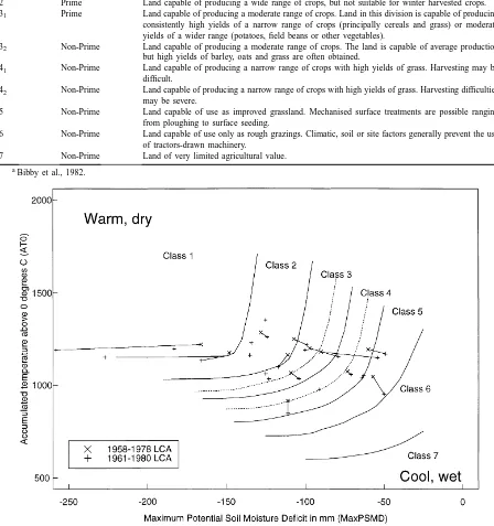
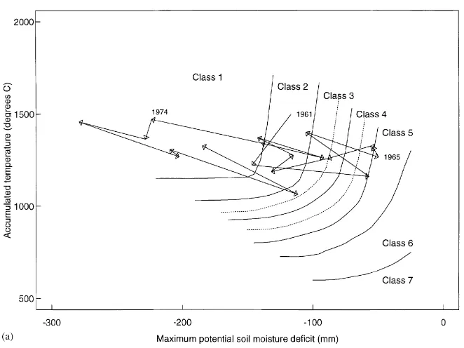
The LCA system (Bibby et al., 1982) was devel-oped for Great Britain by an expert group but was applied only in Scotland. It is based on the concept of flexibility of use of land and was inspired by the work of Klingebiel and Montgomery (1961) in Amer-ica and the FAO (1984). The LCA system comprises seven classes with some sub-divisions, described in Table 1, based on a wide range of land qualities de-rived from topographic, soil and climatic variables. In this study, only the climatic component of the classifi-cation, based on temperature and moisture supply, was considered. There are seven climatic LCA classes, of which two are sub-divided — 1, 2, 31, 32, 41, 42, 5, 6 and 7. The class boundaries in relation to accumu-lated temperature and maximum potential soil mois-ture deficit are shown in Fig. 1.
The climatic LCA classes were constructed using weather data to derive annual values of accumulated temperature above 0◦C (AT0) and median maximum potential soil moisture deficit in mm (MaxPSMD). AT0 was defined as the accumulated sum of de-grees above 0◦C for each day from 1 January to 30 June. MaxPSMD is the theoretical maximum mois-ture deficit under a complete cover of short grass with no limit on water supply, computed by accu-mulating the daily moisture deficit between rainfall and evapotranspiration. The maximum value of the accumulated deficit during the year was used for the general climate classification considered here.
Table 1
Description of Land Capability for Agriculture Classesa
Class Category Description
1 Prime Land capable of producing a very wide range of crops, including winter harvested vegetables. Yields are consistently high.
2 Prime Land capable of producing a wide range of crops, but not suitable for winter harvested crops. 31 Prime Land capable of producing a moderate range of crops. Land in this division is capable of producing
consistently high yields of a narrow range of crops (principally cereals and grass) or moderate yields of a wider range (potatoes, field beans or other vegetables).
32 Non-Prime Land capable of producing a moderate range of crops. The land is capable of average production
but high yields of barley, oats and grass are often obtained.
41 Non-Prime Land capable of producing a narrow range of crops with high yields of grass. Harvesting may be
difficult.
42 Non-Prime Land capable of producing a narrow range of crops with high yields of grass. Harvesting difficulties
may be severe.
5 Non-Prime Land capable of use as improved grassland. Mechanised surface treatments are possible ranging from ploughing to surface seeding.
6 Non-Prime Land capable of use only as rough grazings. Climatic, soil or site factors generally prevent the use of tractors-drawn machinery.
7 Non-Prime Land of very limited agricultural value.
aBibby et al., 1982.
Fig. 1. Partition of median maximum potential soil moisture deficit and lower quartile accumulated temperature above 0◦C into climatic
to compute AT0 and MaxPSMD for each station and year combination. The data were from a non-standard period, 1958–1978. The annual AT0 and MaxPSMD values were summarised for each station, using quar-tile statistics to reduce the impact of extreme values. The lower quartile value of AT0 and the median value of MaxPSMD were used in devising the empirical climatic LCA classification. A plot of lower quartile AT0 against median MaxPSMD for these climate sta-tions was used to draw climatic LCA class boundaries. The class boundaries are shown on Fig. 1, together with the positions of 23 Scottish stations used in this case study. This subdivision of warmth and moisture into LCA classes provides an empirical classification of Great Britain, in terms of the climatic conditions influencing flexibility of cropping.
In Scotland, a simplification of the LCA system for planning purposes was developed in National Planning Guidelines for agricultural land (Scottish Develop-ment DepartDevelop-ment, 1987). In these guidelines, ‘Prime’ (P) land comprises LCA Classes 1, 2 and 31 and ‘Non-Prime’ (NP) land comprises the remaining LCA classes, which have less flexibility in land use. The intention was to identify Prime land and protect it from sterilisation by irreversible development (e.g. building). Although a range of other soil and topo-graphic factors influence the designation of Prime or Non-Prime land, only the climatic limitations are con-sidered in this study.
2.2. Climate data
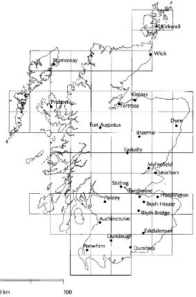
There are no conventions about the length of pe-riod used when summarising climatic data for land evaluation, and in theory any period could be used. In addition, there are no definitive methods for obtaining spatial estimates of weather variables for mapping land classes. The published LCA classification was developed and applied using daily weather data from the period 1958–1978. For the comparison carried out in this case study, limited to Scotland, the LCA classes derived by Bibby et al. (1982) were compared to those derived from the nearest available 20-year reference period, 1961–1980. There are 23 Meteo-rological stations in Scotland for which comparable data were available (Fig. 2). These data are provided by the Meteorological Office within their Rainfall
and Evaporation Calculation System (MORECS), and comprise measured and modelled values for meteorological variables at individual climate sta-tions. As an additional part of the MORECS data, a standard procedure developed by the Meteorological Office (Field, 1983) provides values interpolated from the stations for 40 km×40 km grid squares, on a monthly or weekly basis (Fig. 2).
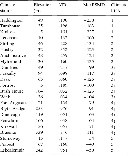
The 1961–1980 MORECS data used in this study were summarised over three different time steps. The station data comprised daily totals of rainfall and evapotranspiration and weekly means of tempera-ture, whereas the 40 km×40 km squares comprised monthly values. The latter are, however, computed by the Meteorological Office from daily observations. At the 23 MORECS stations, we used weekly tem-perature data to compute AT0 (Table 2 and Fig. 2). To compute MaxPSMD, PSMD was computed first, from daily rainfall and evapotranspiration, with
evap-Table 2
Accumulated temperature (AT0) in degrees C, maximum Poten-tial Soil Moisture Deficit (MaxPSMD) in mm and climatic Land Capability for Agriculture (LCA) at the climate stations having Meteorological Office Rainfall and Evaporation Calculation Sys-tem (MORECS) data for 1961–1980
Climate Elevation AT0 MaxPSMD Climatic
station (m) LCA
Haddington 49 1190 −258 1
Turnhouse 35 1196 −183 1
Kinloss 5 1151 −227 1
Leuchars 10 1132 −166 2
Stirling 46 1228 −134 2
Paisley 32 1352 −125 2
Auchincruive 48 1259 −124 2
Mylnefield 30 1160 −135 2
Dumfries 49 1217 −99 31
Stornoway 15 1147 −54 5
Prabost 67 1168 −49 5
Fig. 2. The locations in Scotland of the 23 climate stations and of the Meteorological Office Rainfall and Evaporation Calculation System (MORECS) squares.
otranspiration modelled using the standard method (Penman, 1948) that was used in the published cli-matic LCA classification. Any residual deficit at the end of December was carried forward into the next year. The accumulated daily PSMD values were then used to obtain the MaxPSMD for each year. In the MORECS squares, monthly values of temperature were used to compute AT0 directly, by allocation of
2.3. Risk assessment
In this paper, the interpretation of risk follows that outlined by Warner (1993), who defines risk as the probability that a particular adverse event occurs dur-ing a stated period of time. An adverse event or haz-ard is defined as an occurrence that produces harm, i.e. loss consequent on damage, where damage is the loss of some inherent quality suffered by a physical or biological entity.
Following Warner’s terminology, risk assessment is a general term used to describe the study of decisions subject to uncertain consequences and comprises three stages — risk estimation, risk evaluation and risk man-agement. In this study only risk estimation is covered. To do this, we identified hazard with the Non-Prime land category and estimated the probabilities of oc-currence of the categories Prime and Non-Prime over time. There are a number of ways that such a time series of annual switches between climatic Prime and Non-Prime land can be summarised. For example, the proportion of time spent, or the mean number of con-secutive years in the climatic Prime category could be quoted. In this study, probabilities of occurrence were estimated from the transitions between climatic Prime and Non-Prime land in consecutive years. This is a simple form of Markov-chain analysis and has, for ex-ample, been applied to daily rainfall (Gabriel and Neu-mann, 1962). The transitions between climatic Prime and Non-Prime land are calculated using a sequence of years rather than days (as used for rainfall), but the technique is applied in identical fashion. The principal result is a matrix of transition probabilities. From this matrix, assuming stationarity of the series (no trend), we can estimate two forms of risk: the probability of continuous sequences of years that land is in the cli-matic Prime category and the mean return period in years to climatic Prime land from Non-Prime land.
3. Analyses
Four separate analyses were carried out by allocat-ing 1961–1980 climate data to climatic LCA classes and Prime/Non-Prime categories. First, we compared the climatic LCA for the two periods 1958–1978 and 1961–1980 to test the robustness of the classification. Then we quantified the inter-annual variability from
1961–1980 in climatic LCA class at the MORECS stations. Thirdly, the transition probabilities between climatic Prime and Non-Prime categories were esti-mated. Finally, the geographic variation in mean return times to the climatic Prime category was mapped.
3.1. Effect of different climate periods
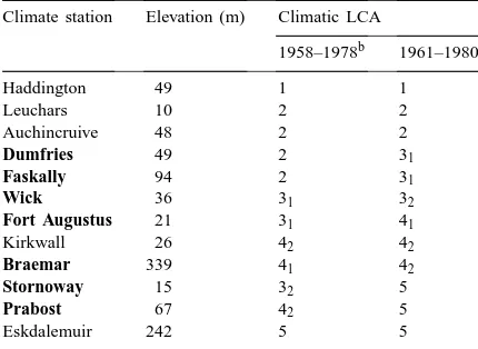
Comparing the climatic LCA classes for the periods 1961–1980 and 1958–1978, we tested the null hypoth-esis that climatic LCA class is not sensitive to the cli-mate period used. Comparable data were available for 12 stations. The climatic LCA classes from 1958–1978 and those derived from 1961–1980 are summarised in Table 3. The climatic LCA class is lower in 1961–1980 than in 1958–1978 for seven of the stations (shown in bold type). Additionally, in Fig. 1, the change in po-sition of each station is shown with a line connecting its position in 1958–1978 to that in 1961–1980. This shows that some stations move more than others do and that there is a general shift to cooler and wetter in most stations. If the second period of data were used to construct the class partitions their positions would be shifted on the graph.
To test the null hypothesis that there was no differ-ence in the LCA class for the two periods, the classes were compared using a randomisation test. For each station, the pair of climatic LCA values (1958–1978
Table 3
Long-term climatic Land Capability for Agriculture for 1958–1978 and 1961–1980a
Climate station Elevation (m) Climatic LCA
1958–1978b 1961–1980
aStations which do not change LCA class are highlighted in
bold.
and 1961–1980) was randomly allocated to the two periods. This gave a randomised set of 12 pairs of climatic LCA classes. The mean difference in cli-matic LCA classes between the two periods was then calculated for this randomised set of 12 pairs. This procedure was repeated a 1000 times to generate a distribution of mean differences which was then com-pared with the observed mean difference. The results showed that there is a 99.5% chance of the stations having different long-term climatic LCA classes.
The result demonstrates that the climatic LCA class is sensitive to the period from which climatic data are selected and the null hypothesis is therefore rejected. The implications for the construction of the climatic LCA class partitions will be discussed later. The inac-curacy arising from using the empirical classification derived with 1958–1978 climate data to allocate LCA classes with the 1961–1980 climate data has minimal impact on the following results.
3.2. Inter-annual variability in climatic LCA
While the land capability system is a long-term classification, it is sensitive to weather variability. We have chosen to quantify that inter-annual variability using climatic LCA. Each year’s MaxPSMD and AT0 were used to allocate the station to a notional an-nual climatic LCA class. For each station, time series of the annual climatic LCA classes and the 20-year trajectory of each station’s AT0 versus MaxPSMD were plotted onto the 1958–1978 climatic LCA class partition of the AT0 and MaxPSMD feature space. Examples are given in Fig. 3a and b for Auchincruive and Braemar. The graphs show that the annual values follow a complex trajectory through the climatic LCA class partitions, such that the long-term climatic LCA class rarely occurs in any individual year, except for stations near each end of the LCA range in Classes 1 and 5. In addition, plotting the trajectories of several stations on a single graph (not shown here) revealed that the relative positions of stations change through time, indicating that the spatial correlation structures are not constant.
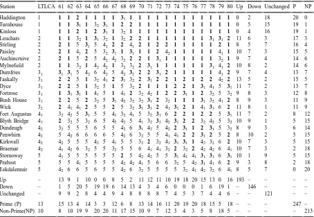
Similar trajectories were plotted for all 23 stations for each year from 1961–1980 and the annual climatic LCA classes read off. These results are presented in Table 4 which also summarises the number of times
the stations are above (+), below (−) or at (=) their long-term climatic LCA class.
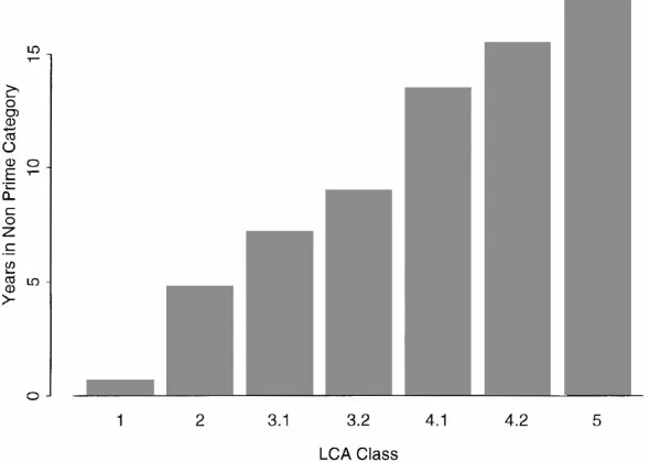
Table 4 can be used to summarise the LCA class and Prime land categories in several ways. For exam-ple, the average time that each climatic LCA class is in the Non-Prime category (Fig. 4) increases for each successive climatic LCA Class from 1 to 5 (for exam-ple, climatic LCA Class 31is in the Prime category for 64% of the 20 years). The results in Table 4 highlight the variability in weather that the climatic LCA class is based on, both between stations and between years. However, they fail to answer the conditional question: ‘After a station leaves a class or category what is the time taken to return to it?’ The answer will establish risk for each station. Markov-chain analysis is used to address this question in the next section, by estimat-ing the mean return time back to a class or category, after leaving it.
3.3. Transition probabilities between land categories
The results mentioned earlier highlight the annual variations in weather that cause the fluctuations in cli-matic LCA class for individual climate stations. Given the number of possible transitions between the nine climatic LCA classes and subclasses, we decided to re-duce the number of classes to two states for estimating transition probabilities. The nine climatic LCA classes were simplified into two broad categories, which have relevance to the study area:
1. climatic Prime category 2. climatic Non-Prime category
Table 4 provides information on those years when the stations were classified in the climatic Prime land category (LCA classes shown in bold) and tabulates the number of times the stations were observed in the climatic Prime/Non-Prime categories.
Table 4
Climatic land capability for agriculture (LCA) for 23 Scottish climate stations computed on an annual basis from 1961–1980a
Station LTLCA 61 62 63 64 65 66 67 68 69 70 71 72 73 74 75 76 77 78 79 80 Up Down Unchanged P NP
aThe long-term LCA (LTLCA) is provided for reference and annual variability is summarised in two ways: (i) instances where annual
LCA is up/down/unchanged relative to the long-term LCA and (ii) the number of instances of Prime (P) vs Non-Prime (NP). Prime land, LCA Classes 31–1, is shown in bold. The summaries reveal variability within stations and between years (rows) and between stations and
within years (columns).
From state P two transitions are possible in a pair of consecutive years; the state can remain the same, i.e. P⇒P or the state can change to NP, i.e. P⇒NP. There are four one-step transitions possible between the two states in two consecutive years, shown in matrix form as
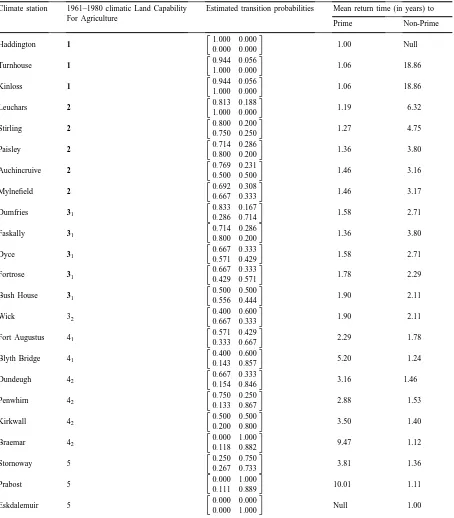
The number of times each of the four transitions oc-cur, is counted at each station and to estimate transi-tion probabilities, proportransi-tions are calculated for each starting state. For example, the matrices of transition counts and probabilities (in brackets) at Auchincruive and Braemar are
Assuming that the sequence of states is stationary (does not display a trend) and manipulating the tran-sition probabilities according to Markov-chain theory (Gabriel and Neumann, 1962), mean return times between states can be estimated.
Table 5
Estimated transition probabilities and mean return times to Prime and Non-Prime land for each climate station in Scotland
Fig. 4. The number of years out of 20 that land at stations is in the Non-Prime category, averaged by land capability for agriculture (LCA) class.
never leaves the Prime state) to null at Eskdalemuir (i.e., never reaches the Prime state). All the stations in climatic LCA Classes 1, 2 and 3 have estimated mrt to Prime land of less than 2 years. Climatic LCA Classes 4 and 5 have mrts to the Prime state of more than 2 years.
As would be expected, the stations classified as be-ing Non-Prime generally have longer mrts. However, the return times do not equate directly to the long-term climatic LCA class (i.e., there is no systematic trend in the mrt from higher to lower climatic LCA class). For example, Stornoway with a long-term climatic LCA Class 5 has a shorter mrt to Prime land than Braemar or Blyth Bridge with climatic LCA Classes 42and 41, re-spectively. These stations are in contrasting geograph-ical locations and it is likely that there is an over-riding spatial structure influencing the climatic variability. This indicates that whilst it is possible to calculate transition probabilities on the basis of climatic LCA class the estimated mrts are a property of the geo-graphic location of the station and not a property of the climatic LCA class. This is a very significant find-ing since it means that the process of interpolatfind-ing these mrt estimates must include explicit account of the spatial and temporal structure of the weather data used to derive the climatic LCA classification.
3.4. Geography of mean return times to Prime land
The preceding section has demonstrated a method for computing mrts to the Prime land category for indi-vidual climate stations. To map the geography of mrts, land evaluation units could be used, as in the approach described by van Lanen et al. (1992). An alternative method, which we have used, is to compute mrts from interpolated weather data. Here, we use Scotland as a case study to illustrate and assess the use of interpo-lated weather data to map mrts over wide geographic areas. The weather data are interpolated to a coarse grid, but the same principle would apply to an inter-polated data set with finer resolution.
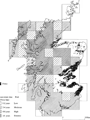
Fig. 5. The mean return times to climatic Prime land in 40 km×40 km Meteorological Office Rainfall and Evaporation Calculation System (MORECS) squares grouped into four risk classes. The Prime land area in Scotland is shown for comparison.
end-of-month MaxPSMD (R2=0.92). The predicted AT0 and MaxPSMD values for each combination of MORECS square and year were then used to allocate the squares to the climatic Prime or Non-Prime cat-egory for each year. Then the mrt to climatic Prime
data and the comparability of climatic Prime land to Prime land, Fig. 5 reveals the broad pattern of varia-tion in mrt or zones of risk, compared to the distribu-tion of Prime land.
This analysis demonstrates that, providing there is an adequate network of meteorological stations and a sufficiently long run of climatic data, it is possible to develop spatial estimates of climatic variability that can be expressed in terms of zones of risk. The climatic LCA methodology can be adapted to incorporate this. So, for example, the mrt to Prime land classes shown in Fig. 5 is re-expressed as low (0–2 years), moderate (2–4 years), high (4–8 years) and extreme (>8 years) risks.
4. Concluding remarks
This study shows the LCA methodology imple-mented in Great Britain is sensitive to the period from which weather data are drawn to develop the classifi-cation. Changes in LCA classes between 1958–1978 and 1961–1980 were found at seven out of 12 stations examined and all 12 stations showed a shift in posi-tion. The general implication of this result for land evaluation is that there is a need to assess the effects of the time period from which weather data are drawn on the construction of class partitions. A secondary point concerns the validity of using a land evaluation system for time periods that extend beyond the base-line weather data period. Whilst these findings could be expected they indicate that work on developing a protocol based on robust methods for incorporating weather variability into land evaluation is necessary. In the meantime, it is worth stressing that LCA class con-struction and subsequent allocation of land to classes should use climatic data from the same period and area, although this is not generally stated in published classifications. Work on robust methods is currently being undertaken, initially by investigating the use of longer reference periods.
Analysis of the inter-annual variability or the time trajectories of individual stations through the AT0 and MaxPSMD feature space reveals that stations rarely occupy their long-term LCA class and that the posi-tions of staposi-tions relative to one another changes from year to year. This suggests that corresponding changes in spatial correlation structures occur. These findings
suggest that more work should be done on analysing the spatio-temporal variability in weather variables used in land evaluation to establish whether groups of stations tend to behave in similar ways over space and through time.
To enable climatic variability to be included in the land evaluation methodology a risk assess-ment approach has been adopted. This is based on Markov-chain analysis of Prime and Non-Prime cat-egories. The estimated mrt to the Prime state was shown to be a property of geographic location rather than the LCA class. The methodology is based on probabilities and several risks could be combined according to the rules for combining probabilities. The Markov-chain approach is generic and could be applied for any dynamic variables used in land evaluation to estimate risk categories.
Mapping zones of risk using interpolated climatic data has extended the approach developed for single stations. The geographical risk is assessed from the interaction between hazard and exposure at a set of places and mapped using interpolation. There are a number of sources of uncertainty in this procedure, arising from the reference climate data period and the density of the climate stations in relation to the weather variability.
The coupling of the Markov-chain analysis and its extension to mapping zones of variability or risk for the Scottish case study indicates that this could form the basis of a formal method for explicitly incorporat-ing weather variability in land evaluation. More work is required to test this in a wider range of climatic con-texts, in terms of climate zone, data availability and investigating temporal variation in other land qualities such as soil wetness.
Acknowledgements
References
Bibby, J.S., Douglas, H.A., Thomasson, A.J., Robertson, J.S., 1982. Land Capability Classification for Agriculture. The Macaulay Institute for Soil Research, Aberdeen.
FAO, 1984. Guidelines: Land Evaluation for Rainfed Agriculture. Soils Bulletin No. 32, Food and Agriculture Organisation of the United Nations, Rome, Italy, 249 pp.
FAO, 1996. Agro Ecological Zoning: Guidelines. Soils Bulletin No. 73, Food and Agriculture Organisation of the United Nations, Rome, Italy.
Field, M., 1983. The Meteorological Office Rainfall and Evaporation Calculation System — MORECS. Agric. Water Manage. 6 (2-3), 297–306.
Gabriel, K.R., Neumann, J., 1962. A Markov chain model for daily rainfall occurrence at Tel Aviv. Q. J. R. Meteorol. Soc. 88, 90–95.
Klingebiel, A.A., Montgomery, P.H., 1961. Land Capability Classification. Agricultural Handbook No. 210, US Department of Agriculture, Soil Conservation Service.
Penman, H.L., 1948. Natural evaporation from open water, bare soil and grass.. Proc. R. Soc. Lond. ser. A Mathematical and Physical Sciences 193, 120–145.
Rossiter, D.G., 1996. A theoretical framework for land evaluation. Geoderma 72 (3-4), 165–190.
Scottish Development Department, 1987. National Planning Guidelines 1987: Agricultural Land. National Planning Series, Scottish Development Department, Edinburgh. 2 pp. van Lanen, H.A.J., Hack-ten Broeke, M.J.D., Bouma, J.,
de Groot, W.J.M., 1992. A mixed qualitative/quantitative physical land evaluation methodology. Geoderma 55 (1-2), 37– 54.