Quality, User Cost, Forward-Looking
Behavior, and the Demand for Cars
in the UK
Jonathan Murray and Nicholas Sarantis
This paper applies an extended version of the superior goods model to the UK car market. The model involves the estimation of separate equations for the demand for new cars and the rental price of used cars. We have allowed for the direct influence of quality on car demand by using a measure derived from hedonic price equations. We have employed three measures of the user cost, reflecting different assumptions about price expectations and the depreciation rate. The empirical results reject the forward-looking model in favor of the error correction formulation. Income, wealth and price elasticities for new and used cars support the superior goods hypothesis. © 1999 Elsevier Science Inc.
Keywords: Demand for cars; Quality; Forward-looking behavior
JEL classification: C5, D12, L62
I. Introduction
It is often said that buying a car is the most expensive purchase that consumers have to make, after housing. The car industry is also one of the major manufacturing industries, and figures on car sales are often used as one of the main business cycle indicators. Despite the importance of the car market to aggregate demand, output and employment,
This paper was presented at the 10th Annual Congress of the European Economic Association, Prague, September 1995. Helpful suggestions by the participants of this conference, two anonymous referees and the editor of this journal are gratefully acknowledged. We are also indebted to K. Cuthbertson, S. Hall, S. Price and R. Smith for their constructive comments on an earlier version of this paper. One of the authors (Nicholas Sarantis) has benefited from a grant from the British Academy.
Energy Saving Trust, London, United Kingdom; Department of Economics, London Guildhall University, London, United Kingdom.
Address correspondence to: Dr. N. Sarantis, London Guildhall University, Department of Economics, 84 Moorgate, London EC2M 6SQ, United Kingdom.
there has been hardly any empirical work on the demand for cars in the United Kingdom.1 To our knowledge, the only study on this topic was a paper in the 1970s by Armstrong and Odling-Smee (1979). Hence, the aim of the present paper is to provide an econometric investigation of the determinants of aggregate demand for cars in the United Kingdom.
The theoretical model employed is the superior goods model proposed by Wykoff (1973) and subsequently used by Johnson (1978) and Tishler (1982).2However, we have made a number of significant extensions to the Wykoff (1973) model. First, we allowed for the direct influence of quality on car demand, by using a measure of quality derived from hedonic price equations. As Trandel (1991) pointed out, omitting quality from a demand regression will lead to biased parameter estimates. Second, we used three alternative measures of the user cost of new cars, which reflect different assumptions about price expectations and the depreciation rate. Third, following Tishler (1982) and Armstrong and Odling-Smee (1979), we allowed for the separate influence of vehicle running costs. In the empirical implementation of the model, we employed the cointe-gration methodology to examine the long-run equilibrium demand for cars, while the short-run dynamics of car demand were examined within the context of both the error correction model and the forward-looking rational expectations model.3This contrasts with all previous studies in this area which used rather ad hoc (mostly static) functional forms.
The paper is organized as follows. In the next section, we set up a theoretical demand model for cars. Section III outlines the modelling methodology. In Section IV, we explain our methodology for deriving a measure of quality for new cars. Section V describes the measurement of the variables and analyzes the empirical results for new car demand. Section VI presents the results for used car rental prices. In the final section, we summarize the main empirical findings.
II. A Model For Car Demand
The basic supposition is that consumers derive utility from the transport services provided by cars. The cost of these services is defined as the user cost, that is, the cost to the user of the car of the transport services provided. For any asset, the user cost is defined as the depreciation of the asset during the period in which the asset is used, plus the opportunity
1In contrast to the UK experience, a number of authors have investigated the aggregate demand for cars in other countries, particularly in the United States. See, for example, Chow (1957), Wykoff (1973), Johnson (1978), Blomqvist and Haessel (1978), Tishler (1982), Levinsohn (1988), De Pelsmacker (1990), Trandel (1991).
2An alternative approach is to estimate structural demand functions for individual car attributes using panel data. These estimates are then used to make inferences about the demand for cars; see, for example, Atkinson and Halvorsen (1984), and Bajic (1993). Although this approach provides useful information to car designers and corporate planners, we do not think it is very helpful for understanding cyclical movements in the car market. The models employed in this area are basically static and fail to capture the influence of important aggregate economic factors (i.e., income, wealth, borrowing costs, etc.) on car demand. The issue of differences in quality raised by this literature is addressed in our paper by deriving a measure of quality based on individual car characteristics. Our theoretical model also differs from the structural approach, which focuses on car ownership growth [see Button et al. (1982)] and is normally found in the marketing literature, as well as from the stock adjustment model which treats both new and used cars as homogeneous goods.
cost of holding that asset in the consumer’s portfolio [Wykoff (1973) and Johnson (1978)].
) is the depreciation of the value of the car during time t; Vt n
is the purchasing price of the new car; V1,t11
ue
is the expected market value of this car in one year’s time on the second-hand market; (rtVt
n
) is the opportunity cost of holding the car during period t, and rtis the interest rate.
Similarly the user cost of a used car, Ut u
is the market value of an s-year old car on the second-hand market, and Vs11,t11
ue
is the expected market value of this second-hand car in a year’s time.
The fact that new cars depreciate on average by 30% in their first year of use, as opposed to used cars which depreciate at a relatively constant rate of 10% in any given year, implies that the user cost of owning a new car is much higher than that of owning a used car. The persistence of this user cost differential in an advanced and competitive car market suggests that there exists added utility in owning the latest model, after which cars join the ranks of used cars and are worth far less. Added to this is that most car owners purchase their vehicle with financial loans, and that at least 40% of new cars are purchased by companies primarily for the use of their employees, so it is reasonable to view car owners as renting the vehicle to themselves. This view is given added weight by the importance of buying a car in August with the latest registration letter to mark it as a new car. Consequently new cars and used cars would appear to be imperfect substitutes, with the services of new cars considered by consumers to be qualitatively superior to the services of used cars.
The UK car market can therefore be modelled by applying the superior goods model developed by Wykoff (1973), and subsequently used by Johnson (1978) and Tishler (1982). This model is based on the above assumption of the superiority of new car services over used car services, which suggests that new car purchases cannot be treated simply as additions to the existing stock of used cars, but rather they reflect the demand for the services of a unique commodity measured separately from the stock of used cars. The existing car stock influences the demand for new cars only through the rental price of used cars.4 Consequently, the model implies that the demand for new and used cars is determined separately, with only the user cost of each good affecting the level of demand for the other good. Wykoff (1973) and Johnson (1978) used a two-equation system to describe the superior goods model:
Dn5D~Y, Un, Uu,!; (3)
Uu5U~Y, Un, K!, (4)
where equation (3) is the demand for new cars; equation (4) is the demand for used cars;
Y is income; Unis the user cost of new cars; Uuis the user cost of used cars, and K is the stock of used cars.
This is a recursive model with the markers for new and used cars modelled separately. Evidence shows that the supply of new cars in the United Kingdom appears to be almost infinitely price elastic. This is a result of car manufacturers choosing to set the price of new cars, and allowing the market to adjust through the level of sales. Therefore, in this model, the new car price is an exogenous variable and the number of registrations is demand-determined. The used car market, on the other hand, works in the reverse manner. The supply of used cars is effectively fixed in the short term to the existing stock of used cars. There will be a flow of new cars coming into the used car market each period, adding to the car parc, while scrapped cars will be depleting the parc. However, the flow of new cars is effectively determined a year in advance, and the rate of scrappage does not appear to have a discretionary component. Therefore the adjustment in the used car market must come through the price of used cars, which suggests that the quantity of cars is exogenous while the price is endogenous. Because equations (3) and (4) are viewed as a recursive model [see Johnson (1978)], we can legitimately concentrate on the demand for new cars only, though we will report the main findings for the determination of used car rental prices as well, in order to test the superior goods hypothesis.5
Application of the superior goods model to the UK car market requires certain extensions which were ignored by previous researchers. The empirical evidence for aggregate consumers’ expenditure indicates that changes in personal wealth, W, exert a strong influence on consumers’ behaviour [e.g., Muellbauer (1994)], so wealth should be included in the demand model for cars.
An important determinant of new car demand is quality. The car market is not a commodity market where the goods sold are identical; there are considerable differences between various car models, which are generally referred to as quality [e.g., Wykoff (1973); Johnson (1978); Atkinson and Halvorsen (1984); Bajic (1993)]. If quality affects significantly the demand for cars, failure to include a measure of quality in the new car demand regression is likely to introduce substantial omitted variable biases. Trandel (1991) has shown that including quality variables in a model of the US automobile market increases the model’s estimated price elasticity by about 80%. In terms of adapting the demand model for new cars to the United Kingdom, there are two possible methods; firstly, to account for car heterogeneity by translating each new car model into a new equivalent (let us say, a Ford Escort equivalent) and each used car into a one-year old equivalent, as in Wykoff (1973) and Johnson (1978). Secondly, to construct a quality index for cars, Qt, and include it directly as an explanatory variable in the demand
equation. The second method is preferred partly because the Wykoff (1973) method is extremely cumbersome and very sensitive to the chosen numeraire [see Johnson (1978)], and partly because it allows a straightforward comparison of the demand equations with and without the quality index.
Another variable likely to influence the demand for cars is the running cost, Pvs. Tishler (1982) showed that when the stock of cars does not appear directly in the consumers’ utility function, and operating costs are substantial, the demand function should include both user costs and operating costs separately. Using the real gasoline price as a proxy for
operating costs, he found that omission of this variable from the aggregate demand function yielded biased parameter estimates. An argument for the inclusion of running costs in the demand function was also made by Armstrong and Odling-Smee (1979). Consequently the demand model for new cars becomes:6
Dt5a01a1Yt1a2Wt2a3Ut
where vtis the error term.
III. Modelling Methodology
Equation (5) represents the long-run equilibrium demand for cars. Hence, the first step was to investigate this equilibrium demand function using cointegration tests. In the second stage, we developed the dynamics of the car demand function. Two alternative dynamic formulations were employed, both of which had to be consistent with the long-run equilibrium demand function.
First, we assumed that economic agents are backward-looking, so the dynamics of the demand function would be captured by the error correction model, which is based on the residuals of the cointegrating relationship.
Second, we assumed that economic agents are forward-looking, rational decision makers, who choose their short-run demand for cars, Dt, so as to minimize the expected
discounted present value of a multi-period quadratic loss function:
L5Et
H
O
i50`
di@a~D
t1i2D*t1i!21b~Dt1i2Dt1i21!2#
J
, (6)where E is the expectations operator conditional on the information setVt21; d is the subjective discount factor (0, d , 1); a and b are positive parameters, and D* is the long-run equilibrium demand given by equation (5). The loss function (6) implies that there are costs associated with being away from equilibrium and with the adjustment of demand.7The solution to this optimization problem [see Cuthbertson (1990)] yields a structural dynamic demand model:
6The extra variables (i.e., w, q and pvs) obviously enter the equation for used car rental prices (4) as well.
New car sales can also be affected by changes in the tax regime. During the sample period 1977–1991, taxation on car purchases consisted of VAT and car tax. Car tax remained constant at 10% throughout the period, but VAT increased twice. The first increase was in June 1979, when VAT on car purchases went up from 10% to 15%, and again in April 1991, when VAT was increased to 17.5%. The latter increase was at the end of the sample period, so it did not matter. With regards to the first increase, we used a dummy variable for 1979Q2, but it proved to be insignificant.
The usual approach to estimating the forward-looking RE model (7) has been to employ a VAR or other autoregressive system to model directly the expectations forma-tion process and then estimate the dynamics simultaneously with the equilibrium vector [Cuthbertson (1990); Cuthbertson and Taylor (1992)]. But as Pesaran (1987) and Callen et al. (1990) pointed out, we do not have a good idea of the correct expectations formation scheme, so misspecification of the expectations model may lead to incorrect rejection of the forward model. Callen et al. (1990) proposed an ingenious procedure for estimating the forward model; they argued that the equilibrium vector estimated by cointegrating methods is an estimate of D*t, and hence can be used directly in the forward equation.
Thus, substituting the fitted values from the cointegrating regression, as estimates of the future long-run path, into the forward model (7) yields:
Dt5lDt211~12l!~12ld!
O
i50
`
~ld!i~D*
t1i!1 «t. (8)
As the future terms in D* are subject to an REH error, equation (8) was estimated with a non-linear instrumental variables (IV) method as in Callen et al. (1990) and Price (1992, 1994). Assuming that the disturbance term,«t, is serially uncorrelated, the non-linear IV
estimates will be consistent and asymptotically efficient [Cuthbertson (1990)].
IV. Deriving a Measure of Quality
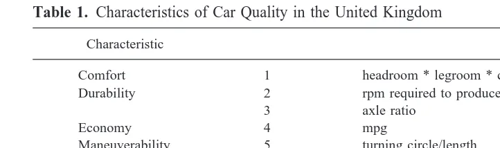
The construction of the quality index is based on the hedonic price analysis for UK cars in Murray and Sarantis (1994). The basic idea of hedonic price theory is that the good car is viewed as a bundle of individual attributes or characteristics, each having its own price determined in a competitive market. It is these characteristics which distinguish different car models and, as such, represent the quality of each vehicle. The quality of a car can then be described in terms of the quantity of a set of characteristics. The individual car characteristics and the variables used to represent these quality characteristics for cars in the UK are shown in Table 1, and are discussed in Murray and Sarantis (1994).
Following Feenstra (1988), we used the Fisher ideal index to construct a quality index based on the estimates of the hedonic price equations reported in Murray and Sarantis (1994). The Fisher ideal index, which is a geometric mean of the Laspeyres and Paasche indexes, used in the construction of the quality index is:
Table 1. Characteristics of Car Quality in the United Kingdom
Characteristic
Comfort 1 headroom * legroom * cabin width
Durability 2 rpm required to produce maximum bhp
3 axle ratio
Economy 4 mpg
Maneuverability 5 turning circle/length
Performance 6 maximum bhp/weight
Safety 7 braking distance
Qnt5
Î
Xt~bˆt21! Xt21~bˆt21!
* Xt~b
ˆt!
Xt21~bˆt!
, (9)
where X is the average level of the jth characteristic in new cars in each quarter, whilebˆ is the estimated marginal value for the corresponding jth characteristic in the same period, reported in Murray and Sarantis (1994).
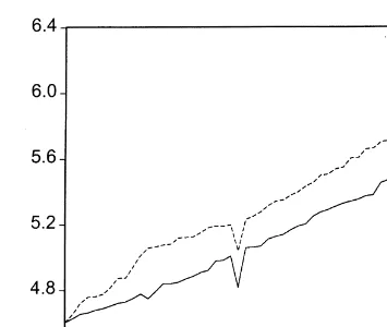
The quality index, together with the average value of new cars, are displayed in Figure 1. It is interesting to observe that the increase in the value of cars during the 1980s was due almost entirely to improvements in quality, which implies that the quality-adjusted real price of cars actually declined during the period 1977–1991. This probably reflects the increasing importance of vehicle specification as an essential selling point for cars in the United Kingdom.
V. Empirical Analysis of the Demand Model for New Cars
The Data
The data used in the estimation of the car demand equation are quarterly from 1977Q1 to 1991Q4. The measurement of variables and data sources are explained in the Appendix, but a few clarifications are deemed necessary here. Following Armstrong and
Smee (1979), the demand for new car purchases is measured by new car registrations rather than sales, because we feel that the data on registrations are more reliable and consistent than those for sales. We would prefer to measure car registrations per house-hold, but due to the lack of consistent quarterly data on the number of households, we have instead expressed car registrations per head. Hence, the income and wealth variables are also per capita measures. Given than at least 40% of new car purchases in the United Kingdom are company fleet purchases, we measured income by real national income rather than by personal disposable income.8
We used three measures for the user cost of new cars. Following Wykoff (1973), we replaced the expected price of new cars in a year’s time on the second-hand market by the actual price that is realized the next year. This produces an ex post user cost, Unp, given by:
Unpt 5~Vtn2Vu1,t11!1rtVtn. (10)
Johnson (1978) proposed the use of the adaptive expectations scheme and argued that, on empirical grounds, the expectations elasticity is unity for the real car price. As a result, the expected second-hand value of the new car is replaced by the current price of an s1 1 year old car. This produces an ex ante measure of the user cost, Ut
na
,
Utna5~Vtn2Vtu!1rtVtn. (11)
Both these measures assume a variable depreciation rate over time. An alternative assumption, often employed in the literature on fixed investment, is that of a constant depreciation rate,g. This gives us a third measure, Ut
nc
, obtained from:
Utnc5Vtn~gn1rt!. (12)
In the case of used cars, past evidence shows that after their first year, cars tend to depreciate at a relatively constant rate. Wykoff (1973) made a similar argument for the US car market. Therefore, the user cost of new cars is measured by:
Utu5Vtu~gu1rt!. (13)
Following previous studies in this area, all rental prices are divided by the consumer price index to ensure homogeneity in money income and prices.
Running costs is another problematic variable. Armstrong and Odling-Smee (1979) proposed the use of total (real) running cost, while Tishler (1982) recommended the use of the real price for petrol and oil. However, neither of these variables made any difference to the cointegration tests, and their coefficients in the error correction model were entirely insignificant and often wrongly signed.9The third variable that we tried was the real price of motor vehicle services (see Appendix). This strongly outperformed all other measures of running costs; hence, all reported empirical findings are with this measure.
8This issue was acknowledged by Armstrong and Odling-Smee (1979) as well, but in the empirical implementation of their model, the authors did not allow for the influence of business income, due to the unavailability of consistent quarterly data on company profits. We think that this problem can be overcome by using national income per capita instead of personal income per capita.
Long-Run Equilibrium Demand Equations
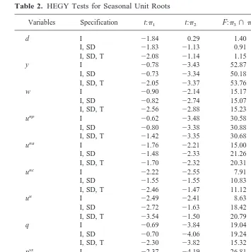
Inference in the cointegration approach is conditional on the order of integration of the variables. As most variables are not seasonally adjusted, we tested for both seasonal and autoregressive unit roots. A seasonal economic time series { xt} is said to be integrated of
order (i, j), i.e., xt3I(i, j), if the series becomes stationary after one-period differencing
(unit root) and seasonal differencing j times (seasonal unit root). To test for seasonal unit roots, we applied the tests recently proposed by Hylleberg et al. (1990), hereafter referred to as the HEGY test. The HEGY statistics for all variables, measured in natural logarithm (indicated by the use of lower-case letters), are shown in Table 2. The test,p150, is for a unit root; the test,p250, is for bi-annual stochastic seasonality, and the joint test for
p3andp4tests for annual stochastic seasonality. Hence, rejection of stochastic seasonality requires rejection of the last two hypotheses. The t statistic forp2and the F statistic for the joint test,p35p4, suggest that five variables contain seasonal unit roots; i.e., d, w, Table 2. HEGY Tests for Seasonal Unit Roots
Variables Specification t:p1 t:p2 F:p3ùp4 LM(4) m
una, unc and uu. The F statistic indicates that the variable, d, has annual seasonality, whereas the other four variables have bi-annual seasonality. It should be noted that these results hold, irrespective of the deterministic terms added, and the seasonal dummies are broadly insignificant. Hylleberg et al. (1990) suggested filtering out the seasonal unit roots and testing for cointegration with the filtered series. Time series with annual seasonality are filtered by (11L1L21L3), while those with bi-annual seasonality are filtered by (11L).
To test for autoregressive unit roots, we employed the Augmented Dickey-Fuller test [see Dickey and Fuller (1979)]. In the case of variables with stochastic seasonality, we applied the ADF test to the filtered series. The conclusion drawn from the ADF statistics in Table 3 is that all variables are I(1). These results are broadly similar to those implied by thep1tests reported in Table 2 and, therefore, all series can enter into cointegrating relationships.
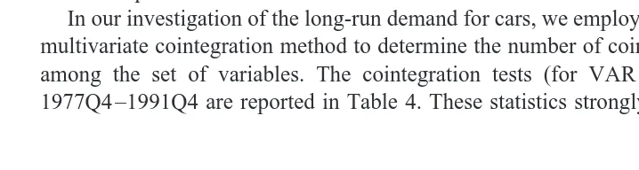
In our investigation of the long-run demand for cars, we employed the Johansen (1988) multivariate cointegration method to determine the number of cointegrating relationships among the set of variables. The cointegration tests (for VAR 5 2), for the period 1977Q4 –1991Q4 are reported in Table 4. These statistics strongly support the existence Table 3. The Augmented Dickey-Fuller (ADF) Test for Unit Roots
Variables
Notes: The 5% critical value for testing the significance of the ADF statistic is approximately22.9 [Dickey and Fuller (1979)]. The numbers within parentheses are the lagged dependent variables in the ADF regression.
Table 4. Johansen Maximum Likelihood Test for Cointegration (22InQ): Demand for New Cars
z50 56.336 62.919 64.718 46.455
z,51 31.412 38.005 37.404 40.303
z,52 28.338 25.253 26.549 34.400
z,53 24.985 21.496 22.156 28.138
z,54 18.028 19.722 18.618 22.002
of one significant cointegrating vector, irrespective of the measurement of the user cost.10 The respective cointegrating vectors are:
d521.80912.319y20.904w20.880unp10.864uu11.082q28.389pvs; (14a)
d542.82910.031y21.618w21.188una12.455uu13.720q213.759pvs; (14b)
d531.02211.669y21.307w23.074unc13.208uu12.715q210.746pvs. (14c)
All the coefficients have the anticipated sign except the one on wealth. Attempts to exclude wealth from the cointegrating vector were rejected by the likelihood ratio test. Looking at the size of these coefficients, however, most of them seem to be exceptionally large and implausible as long-run demand elasticities. Furthermore, they vary consider-ably depending on the measurement of the user cost, with the income elasticity ranging from 2.319 to 0.031. As Cuthbertson and Gasparro (1993) pointed out, misspecification in the arbitrary equations for the VAR, other than that for car demand, may contaminate the long-run elasticities of the demand equation. We, therefore, decided to estimate the unique cointegrating relationships with the Engle and Yoo (1991) three-step method to see whether we could improve on the above long-run elasticities. The advantage of this procedure over the Engle and Granger (1987) cointegration method is that it provides asymptotically efficient estimates of the cointegrating parameters and their standard errors; hence, it allows inference on the long-run car demand equations.11The estimates of the cointegrating relationships (with corrected t statistics in parentheses) are:
d528.94413.252y20.847w20.209unp10.439uu10.219q22.641pvs;
~1.8! ~5.7! ~4.8! ~2.9! ~4.6! ~1.8! ~3.7! (15a)
d529.24513.271y20.907w20.262una10.474uu10.261q22.673pvs;
~1.9! ~6.8! ~6.1! ~4.6! ~5.8! ~2.0! ~4.0! (15b)
d528.93813.534y20.922w20.897unc10.867uu10.316q22.705pvs.
~1.9! ~7.6! ~6.4! ~4.9! ~6.4! ~2.4! ~4.1! (15c)
The signs of the coefficients are the same as those in equations (14a)–(14c), but the inconsistency mentioned above has now disappeared; the parameter estimates are very similar, irrespective of the measurement of the user cost,12 statistically significant, and seem quite plausible as long-run demand elasticities. An important finding is the
signif-10We also investigated the importance of financial liberalization in the 1980s, by employing two variables: the ratio of total consumer credit (net lending) to GDP, and the ratio of UK banks’ lending to private sector to GDP. However, neither of these variables made any difference to the cointegration results, and their coefficients in the error correction model were entirely insignificant, with t values well below unity. This might reflect the fact that hire purchase restrictions on new cars were abolished in 1977. Furthermore, company fleet sales represent a large proportion of new cars, and companies might not face similar credit constraints as private car owners. Notice that the estimation of the Johansen cointegrating system was done with Microfit 3, which does not report standard errors for the cointegration coefficients.
11For a good explanation and application of the Engle and Yoo (1991) three-step cointegration method, see Patterson (1994). An alternative approach is to estimate directly a non-linear error correction model which incorporates the equilibrium equation, as in Cuthbertson and Gasparo (1993) and Price (1994). However, given the large number of variables in our model and the relatively small sample, we felt that the long-run parameter estimates produced by this approach would have been less accurate and efficient than those produced by the Engle and Yoo (1991) procedure, which is asymptotically equivalent to FIML.
icant and positive relationship between the user cost of used cars and the demand for new cars, which is the expected result for substitute goods predicted by the superior goods hypothesis. As a further check, we initially developed error correction models based on the residuals from the Johansen (1988) cointegrating vectors and the Engle and Yoo (1991) cointegrating vectors, respectively. The former were systematically inferior to the latter, both on the basis of the usual econometric statistics and on formal non-nested tests, irrespective of the measurement of the user cost for new cars. Similar results were obtained from our experiments with the forward-looking model. We have, therefore, chosen the cointegrating vectors (15a)–(15b) as the representative long-run demand equations for new cars.
Backward-Looking Demand Model
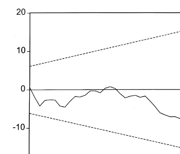
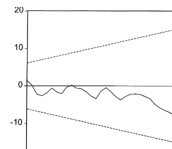
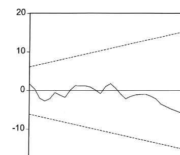
The error correction formulation of the demand model (stage two of the Engle and Yoo (1991) procedure) was estimated with the OLS method over the period 1978Q2–1990Q4, leaving four quarters for ex-post prediction tests.13Testing down from a general equation has produced the results shown in Table 5. The statistics for autocorrelation, heteroske-dasticity, functional form and normality are well below their respective critical values, irrespective of the measurement of the user cost, so there is no indication of misspecifi-cation. The tests for ex-post forecasting performance and structural break strongly support parameter stability for all regressions. This finding was re-enforced by the CUSUM tests of recursive residuals displayed in Figures (2)–(4).14We notice that the lagged cointe-grating residuals display the anticipated negative sign and are statistically significant (even at the 1% level of significance) in all regressions, which provides further support for the ECM specification. The small coefficients on the error correction terms suggest that new car demand adjusts rather slowly towards its long-run equilibrium level.
The ex post user cost for new cars is highly insignificant and wrongly signed, which is in line with a similar result obtained by Johnson (1978) for the United States. On the other hand, both the ex ante user cost and the constant depreciation user cost for new cars exerted a strong (even at the 1% level of significance) negative effect on the demand for new cars, though these elasticities are smaller than the estimates reported by Wykoff (1972), Johnson (1978) and Tishler (1982). Apart from employing a different specification for the dynamic demand model and covering a different sample period and country, one potential explanation for the smaller elasticities might be the finding of a negative and strong effect from motor vehicle servicing costs. It is well known that insurance, repairs and other vehicle servicing costs rose sharply during the 1980s, so operating costs might have become more important than the rental price in deciding whether to purchase a new car. As Armstrong and Odling-Smee (1979) pointed out, higher running costs mean that more income is allocated to current motoring expenses and, hence, less finance is available for replacing the existing car.
13The estimation period commences in 1978Q2, due to the filtering of some variables for seasonal roots (see Section V, second subsection) and the use of lagged variables. Notice that we also introduced seasonal dummies, but these were entirely insignificant, so they were omitted from the final regressions.
An interesting finding is the significant and positive effect of the user cost for used cars, which contrasts sharply with the insignificant effect obtained by Johnson (1978) and Tishler (1982). This cross-price elasticity, however, is well below unity, which implies imperfect substitutability between new and used cars. Our findings remained robust even when the user cost for new cars was deleted, so the possibility of multicollinearity between the rental prices for new and used cars accounting for this result is discounted. The quality index displays the anticipated positive influence and is statistically significant. This finding confirms the importance of quality for car demand regressions as advocated by Trandel (1991). As regards the other variables, we notice that both income and wealth exerted a highly significant and positive effect on the short-run demand for new cars. The short-run income elasticity is approximately half the size of the estimates reported by Armstrong and Odling-Smee (1979) and Tishler (1982), but more in line with those obtained by Johnson (1978).
Comparing the three regressions, it is apparent that the ECM obtained with the ex post user cost is inferior to the other two, not only because of the insignificance of the user cost for new cars but also in terms of explanatory power. This result is confirmed by the formal non-nested tests reported in Table 6. The null hypothesis that the ECM with the ex post user cost is the true model was strongly rejected against both alternatives. On the other hand, the null hypothesis that the ECM with the constant depreciation user cost is the true Table 5. Error Correction Specification of the Demand for New Cars
1. Ex Post User Cost for New Cars (M1)
Ddt520.00611.165Dyt10.322Dwt2210.039Dut 0.438, ARCH(1)50.054, FOR(4)56.715, STAB(24, 18)50.629
2. Ex Ante User Cost for New Cars (M2)
Ddt520.00611.228Dyt10.346Dwt2220.146Dut 0.537, ARCH(1)51.164, FOR(4)54.829, STAB(24, 18)50.511
3. User Cost for New Cars with Constant Depreciation Rate (M3) Ddt520.00611.304Dyt10.380Dwt2210.588Dut 0.173, ARCH(1)50.383, FOR(4)53.716, STAB(24, 18)50.456
Notes: Estimation period 1978Q2–1990Q4; RES is the cointegrating residuals; R2is the coefficient of determination adjusted
for degrees of freedom; SER is the standard error of the regression; LM is the Lagrange Multiplier test for serial correlation up to jth order [x2(j)]; RESET is Ramsey’s reset test for functional form [
x2(1)]; BJ is the Bera-Jargue test for normality [
x2(2)];
HET is the Lagrange Multiplier test for heteroskedasticity [x2(1)]; ARCH is the autoregressive conditional heteroskedasticity test
[xs
2(1)]; FOR is the CHOW test for ex-post predictive failure up to four periods [
x2(4)]; STAB is the CHOW structural stability
test [F(v1, v2)], sample split 1984Q4; DUM is a dummy variable which takes the value of 1 in 1980Q2, and zero elsewhere;
model was easily accepted against the other alternatives, but the converse did not apply.15 Hence, regression M3 is our preferred ECM model for the dynamic new car demand.
Forward-Looking Demand Model
The fitted values of the cointegrating equations (15a)–(15c) were incorporated into the forward-looking specification of the dynamic demand model. Direct estimation of this model by non-linear IV over the period 1978Q2–1990Q4 produced the results shown in Table 7.16 The maximum lead was four, as higher leads were entirely insignificant. Following Pesaran (1992), we also report t values adjusted for White’s heteroskedasticity-consistent standard errors. The Box-Pierce statistics indicate absence of residual autocor-relation for all regressions, so the IV estimates are consistent and efficient. Sargan’s test supports the independence of instruments used in the estimation of the regressions. The
15During the 1980s, a great number of small car-hire companies went bankrupt, while larger fleet operators incurred large financial losses because their cash flows and profitability were too dependent on the residual value of their fleets. Typically, fleet operators had used a constant depreciation rate to determine the expected residual value of their fleets, and it is understood that this was a major factor for their financial losses. Hence, our empirical support for the constant depreciation-based user cost reflects that evidence.
statistics for functional form, normality and heteroskedasticity are also well below their corresponding critical values, though the formulae for these statistics are not very accurate for non-linear estimation methods and should therefore be treated with caution. The parameter,l, is highly significant, positive and significantly smaller than unity as required by the solution to the multi-period optimization problem. On the other hand, the discount parameter, d, is numerically very small and entirely insignificant (with a t value well below unity). Identical results were obtained with White’s heteroskedasticity-consistent standards errors.
To get some idea of the validity of the forward model, we needed to test it for parameter constancy and against clearly-defined alternatives. The Hendry ex post forecast test for the period 1989Q1–1990Q4 (shown in Table 7) was well above its critical value in the regressions with ex post and ex ante measures of user cost; while in the case of the constant depreciation-based user cost, it was on the borderline. This evidence suggests serious parameter instability and inferiority to the ECM regressions.17
17Given that our sample period ends in 1991Q4, and that we used four lead periods, we could not carry out ex post forecast tests beyond 1990Q4. We have therefore re-estimated the forward model over the 1978Q2– 1988Q4 period, and used it to produce ex post forecasts for the period 1989Q1–1990Q4 [see Cuthbertson (1990) for a similar approach]. We also produced ex post forecasts for four quarters (1990Q1–1990Q4), but the Hendry forecast statistics were still well above their critical value for all regressions, thus confirming parameter instability.
To test the REH restrictions implied by the theory, we estimated the unrestricted version of the forward model (8). The forward convolution of all three regressions was poorly determined, which is in line with a similar result reported by Callen et al. (1990) and Price (1992, 1994). The quasi likelihood ratio tests of the forward restrictions were
x2(4) 57.06,x2(4)5 1.96 andx2(4)5 1.24, respectively, for the models based on the ex post, ex ante and constant depreciation user cost. So, the forward restrictions are easily accepted for all estimates.
Another important comparison is with the backward-looking error correction model (ECM) reported in Table 5. As the two models are non-nested, we followed Price (1992)
Figure 4. Cumulative sum of recursive residuals (Model M3).
Table 6. Non-Nested Tests for Error Correction Models
H0 H1
Encompassing Test
[F(2, 40)] J Test
and Cuthbertson and Taylor (1992) in using the IV version of the J test proposed by Mackinnon et al. (1983). To make sense of the tests, we compared the forward and ECM models based on the same measure of the user cost as reported in Tables 7 and 5, respectively. The results are summarized in Table 8. The null hypothesis that the ECM model is the true model was easily accepted against the alternative of the forward model, irrespective of the measure of user cost employed. On the other hand, the null hypothesis that the forward model is the true model was strongly rejected against the alternative of the ECM for all three measures of the user cost. This unambiguous finding about the superiority of the ECM model over the forward model contrasts with the more mixed results reported by Price (1992) for producer prices, and Cuthbertson and Taylor (1992) Table 7. Estimates of the Forward-Looking Dynamic Demand Model (8)
1. Ex Post User Cost for New Cars
l5 0.726 d 5 0.314
(12.98) (0.7)
[11.8] [0.9]
R250.973, SER50.022, BP(1)52.976, BP(4)55.914, BP(6)57.057, RESET(1)50.212, BJ(2)51.045, HET(1)5
1.493, HF(8)526.604, SIV(12)516.636
2. Ex Ante User Cost for New Cars
l5 0.680 d 5 0.290
(12.4) (0.8)
[10.4] [0.9]
R250.979, SER50.019, BP(1)50.803, BP(4)52.868, BP(6)53.633, RESET(1)50.758, BJ(2)51.265, HET(1)5
2.723, HF(8)519.074, SIV(12)515.531
3. User Cost for New Cars with Constant Depreciation Rate
l5 0.680 d 5 0.312
(12.5) (0.9)
[10.7] [1.0]
R250.979, SER50.019, BP(1)50.857, BP(4)53.188, BP(6)53.748, RESET(1)50.504, BJ(2)50.581, HET(1)5
3.684, HF(8)514.877, SIV(12)515.304
Notes: BP(i) is the Box-Pierce statistic for autocorrelation up to ith order; (..) is the conventional t value; [..] is White’s Heteroskedasticity-consistent t value; SIV(..) is Sargan’sx2statistic for the independence of instruments. The other diagnostic
statistics are explained in Table 5.
Table 8. Non-Nested Tests: ECM vs Forward-Looking Model
H0 H1 Test*
1. Ex Post User Cost for New Cars
ECM Forward model 0.411
Forward model ECM 2.524
2. Ex Ante User Cost for New Cars
ECM Forward model 0.201
Forward model ECM 3.782
3. User Cost for New Cars with Constant Depreciation Rate
ECM Forward model 0.133
Forward model ECM 3.659
for the demand for money, but agrees with a similar finding by Price (1994) for UK manufacturing employment.
VI. Results for Used Car Rental Prices
In order to test the superior goods hypothesis, we also examined the determination of rental prices for used cars (equation (4)). Following the same procedure as for new car demand, we estimated cointegrating and error correction regressions using all measures of new car user cost. The estimates obtained with ex post and ex ante user cost were considerably inferior (in terms of the usual diagnostic criteria outlined above) to those obtained with the constant depreciation user cost. This result is similar to that obtained for new cars, and it might suggest that consumers display myopic behaviour as far as car purchases are concerned. Hence, due to space constraints, we only report the results based on the latter measure of new car user cost. The Johansen (1988) test supported the presence of a unique cointegrating vector [LR( z50)582.4,xc
25
46.5, and LR( z,5 1)5 38.6, xc
25
40.3]. The respective long-run equilibrium estimates (with corrected t statistics) and the error correction formulation (with dummies for outliers in 1980Q2, 1986Q3, 1990Q2) of equation (4) are:
uu523.65111.126y10.108w11.269unc20.772q20.114pvs20.588k;
~0.4! ~1.7! ~0.4! ~10.3! ~4.7! ~0.1! ~1.1! (16)
Duu50.01310.211Dw
t11.208Dutnc20.498Dunct2110.745Dptvs21
~2.0! ~2.1! ~12.7! ~3.8! ~2.8!
(17)
21.657Dkt2110.509Dutu2120.151Dutu2220.227RESt211dummies,
~2.0! ~6.0! ~2.8! ~4.4!
R250.901, SER50.016, LM~4!54.607, RESET~1!53.72, BJ~2!
53.351, HET~1!50.505, ARCH~1!51.683, FOR~4!53.917
The specification of the dynamic equation (17) is supported by the diagnostic statistics for the disturbance term and parameter stability, and the regression has a high explanatory power. All coefficients are highly significant and display the anticipated signs, except those on income and quality of new cars. The last two variables had a t value well below unity in all experimentations and, hence, were deleted from the final regression. Our findings contrast sharply with Wykoff (1973) and Johnson (1978), who were unable to find any well-specified regression for used car rental prices. They also failed to find significant cross-price effects. Our results indicate a significant cross-price effect, but this is smaller than unity (0.70), thus indicating imperfect substitution. The small coefficient on the cointegrating residuals suggests very slow adjustment towards equilibrium. The estimates of the long-run price equation (16) show that used car rental prices are essentially influenced by the user cost and quality of new cars, and to a small extent by income, in the long run.
test wasx2(8)512.37). A test for serial correlation was rejected, though the Box-Pierce statistics were close to the borderline (BP(4)59.02, BP(6)59.67). The forward-looking model, however, was strongly rejected by the error correction model. On the basis of the non-nested test, J, the predictions of the forward-looking model failed to make any improvement on the error correction model ( J50.42), while the predictions of the latter significantly improved the forward model ( J 53.95).
VII. Conclusions
We have developed and applied an extended version of the superior goods model to the UK car market. This model involves the estimation of separate equations for the demand for new cars and the rental price of used cars. The cointegration tests support the existence of unique long-run equilibrium equations for new car demand and for used car rental prices. A striking finding for both new car demand and used car rental prices is the strong rejection of the forward-looking rational expectations model in favor of the backward-looking error correction model, irrespective of the measure of user cost employed. The forward model also showed parameter instability and the estimates of the discount rate were not entirely in line with the predictions of the theory. Furthermore, all the results obtained with the ex post user cost, which is based on the assumption of perfect foresight, were consistently inferior to those obtained with other measures of user cost. So, our findings are evidence that UK economic agents behave in a backward rather than forward manner, at least as far as car purchases are concerned.
Overall, the best results for the dynamic demand model for new cars were obtained by the error correction formulation based on the user cost for new cars with a constant depreciation rate. This model passed a wide range of diagnostic statistics and non-nested tests, so it is fairly robust. The results show that quality and user cost for both new and used cars influence significantly the demand for cars, with the user cost for new and used cars displaying negative and positive effects, respectively, as predicted by the superior goods model. An important finding is the strong negative effect of motor vehicle service costs, with a unit elasticity in the short run and an elasticity of approximately22.0 in the long run, which probably reflects the rising insurance premia and other vehicle servicing costs during the 1980s.
Appendix
Data
New Car Registrations (D). New car registrations differ from sales of new cars in a
number of respects. First, the Ministry of Defense (MOD) has a separate registration system to that of the Ministry of the Environment, which is the source of the Society of Motor Manufacturers and Traders (SMMT) data. Secondly, there are grey imports/ exports, which are vehicles purchased in one country and exported/imported by individ-uals. Therefore, registrations do not include vehicles sold to the MOD nor those imported by individuals to the United Kingdom, while they do include vehicles exported by individuals to other countries from the United Kingdom. However, owing to manufac-turers’ restrictive practices, grey imports to the United Kingdom are relatively insignifi-cant, while the demands of the MOD are restricted to particular vehicles, most notably Land Rovers. Total new car registration statistics are taken by the SMMT from the vehicle registration documents collected by the Driver and Vehicle Licensing Authority (DVLA). The data is collected daily and identifies the individual model, engine size and trim specification, and is published in the SMMT’s Monthly Statistical Bulletin. The data used here is quarterly and taken from summing monthly new car registration data. These were divided by total population.
Prices of New (Vn) and Used (Vu) Cars. There is no index or other measure of the price
of new or used cars which is publicly available in the United Kingdom, so we had to construct our own series for the weighted average value (in £) of new and used cars. The data used for new car prices is the recommended retail price of new cars as reported by the car manufacturers. This will tend to introduce some upward bias, as actual transaction prices are likely to be lower than the list price of cars. However, there are no data on the discounts offered by the retailers and, hence, on the actual transaction prices. The data for used car prices are the reported hand values of one-year old cars. These second-hand market values, which were taken from the Motorist’s Guide to New and Used Car
Prices, published by Blackfriars Press Ltd, are weighted by the volume of new car
registrations of each model when originally purchased.
Running Cost (Pvs). The CSO made available to us quarterly data on consumer
expenditure covering motor vehicle services (i.e., licences, insurance, repairs, spares, AA and RAC subscriptions, imputed value of the use of company cars, and other costs), petrol and engine oil. These data are seasonally adjusted at current and constant values; hence, we were able to derive implicit price indexes for total running cost, petrol and engine oil, and motor vehicle services, all divided by the consumers’ price deflator (19855100) to produce real prices of running costs. As explained in the first subsection of Section IV, the variable Pvs is measured by the cost of motor vehicle services in the empirical results reported.
Quality of Cars (Qn). The quality index for cars was derived from hedonic price
Stock of Cars (K). Total number of cars in use (parc) per capita. Data for parc were
obtained from SMMT. The measure used from 1982 onwards has an adjustment to take account of vehicle licence avoidance, while earlier measures did not have such an adjustment. To make the series of car parc consistent, the pre 1982 data were inflated by 10%.
Income (Y). For reasons explained in the first subsection of Section IV, this is
measured by gross domestic product at factor cost per capita (at 1985 prices), seasonally adjusted (Economic Trends Annual Supplement 1993).
Wealth (W). This is the sum of net financial and real wealth of the household sector.
Data on financial wealth were obtained from Financial Statistics (various issues). Net real wealth is measured by the total of tangible assets appearing in the CSO Blue Book (various issues). Data were converted to 1985 prices using the consumers’ price deflator, and divided by total population to obtain per capita real wealth.
Interest Rate (r). This is measured by the 3-month interbank rate (Financial Statistics
(various issues)).
The constant depreciation rates for new cars (gn) and used cars (gu) were set at 30% and 10%, respectively, for reasons explained in Section II.
All the variables used in the econometric investigation were measured in natural logarithms and these are indicated by lower case letters.
References
Armstrong, A. G., and Odling-Smee, J. C. August 1979. The demand for new cars II—An empirical model for the UK. Oxford Bulletin of Economics and Statistics 41(3):193–214.
Atkinson, S. E., and Halvorsen, R. August 1984. A new hedonic technique for estimating attribute demand: An application to the demand for automobile fuel efficiency. Review of Economics and
Statistics 66(3):417–442.
Bajic, V. April 1993. Automobiles and implicit markets: An estimate of a structural demand model for automobile characteristics. Applied Economics 2(4):541–551.
Blomqvist, A., and Haessel, W. August 1978. Small cars, large cars and the price of gasoline.
Canadian Journal of Economics 11(3):470–489.
Button, K., Pearman, A., and Fowkes, A. 1982. Car Ownership Modelling and Forecasting. Aldershot, UK: Gower Publishing Company.
Callen, T. S., Hall, S. G., and Henry, S. G. B. September 1990. Manufacturing stocks: Expectations, risk and cointegration. Economic Journal 100(402):756–772.
Chow, G. 1957. The Demand for Automobiles in the United States. Amsterdam: North-Holland. Cubbin, J. 1975. Quality change and pricing behaviour in the United Kingdom car industry
1956–1968. Economica 47:43–58.
Cuthbertson, K. May 1990. Rational expectations and export price movements in the UK. European
Economic Review 34(5):953–969.
Cuthbertson, K., and Gasparro, D. November 1993. The determinants of manufacturing inventories in the UK. Economic Journal 103(421):1479–1492.
De Pelsmacker, P. May 1990. A structural model of the demand for cars in Belgium. Applied
Economics 22(5):669–686.
Dickey, D. A., and Fuller, W. A. 1979. Distribution of the estimators for autoregressive time series with a unit root. Journal of the American Statistical Association 74(366):427–431.
Engle, R. F., and Granger, C. W. J. March 1987. Cointegration and error correction: Representation, estimation and testing. Econometrica 55(2):251–276.
Engle, R. F., and Yoo, B. S. 1991. Cointegrated economic time series: An overview with new results, 237–266. In Long-Run Economic Relationships (R. F. Engle and C. W. J. Granger, eds.). Oxford: Oxford University Press.
Feenstra, R. C. February 1988. Quality change under trade restraints in Japanese autos. Quarterly
Journal of Economics 103(1):131–146.
Hylleberg, S., Engle, R. F., Granger, C. W. J., and Yoo, B. S. 1990. Seasonal integration and cointegration. Journal of Econometrics 44:215–238.
Johansen, S. 1988. Statistical analysis of cointegrating vectors. Journal of Economic Dynamics and
Control 12(2/3):231–254.
Johnson, T. R. June 1978. Aggregation and the demand for new and used automobiles. Review of
Economics Studies 45(3):311–327.
Levinsohn, J. 1988. Empirics of taxes on differentiated products: The case of tariffs in the U.S. automobile industry, 11–40. In Trade Policy Issues and Empirical Analysis (R. E. Baldwin, ed.). Chicago: University of Chicago Press.
Mackinnon, J. G., White, H., and Davidson, R. 1983. Tests for model specification in the presence of alternative hypotheses. Journal of Econometrics 21:53–70.
Muellbauer, J. Summer 1994. The assessment: Consumer expenditure. Oxford Review of Economic
Policy 10(2):1–41.
Murray, J., and Sarantis, N. 1994. Price-quality relations and hedonic price indexes for cars in the United Kingdom. Economics Discussion Paper 94/3. Kingston University. Forthcoming in the
International Journal of the Economics of Business.
Patterson, K. D. October 1994. Engle and Yoo Three-Step Estimation of Consumers’ Expenditure and Housing Equity Withdrawal. Bulletin of Economic Research 46(4):275–288.
Pesaran, M. H. 1987. The Limits to Rational Expectations. Oxford: Basil Blackwell.
Pesaran, M. H. May 1991. Costly adjustment under rational expectations: A generalisation. Review
of Economics and Statistics 73(2):353–358.
Price, S. May 1992. Forward looking price setting in UK manufacturing. Economic Journal 102(412):497–506.
Price, S. August 1994. Aggregate uncertainty, forward looking behaviour and the demand for manufacturing labour in the UK. Oxford Bulletin of Economics and Statistics 56(3):267–283. Tishler, A. May 1982. The demand for cars and the price of gasoline: The user cost approach.
Review of Economics and Statistics 64(2):184–190.
Trandel, G. A. August 1991. The bias due to omitting quality when estimating automobile demand.
Review of Economics and Statistics 73(3):522–552.
Wykoff, F. C. July 1973. A user cost approach to new automobile purchases. Review of Economic