*Corresponding author.
E-mail addresses: [email protected] (W. Blankenau), [email protected] (M. Ayhan Kose), [email protected] (K.-M. Yi).
夽
We thank Narayana Kocherlakota, Simon Potter, and two anonymous referees for helpful comments. We also bene"ted from the suggestions of seminar participants at Clark University, the 1999 Southeast International Economics Conference, and the 1999 Computing in Economics and Finance Conference. The views expressed in this paper are those of the authors and are not necessarily re#ective of views at the Federal Reserve Bank of New York or the Federal Reserve System.
25 (2001) 867}889
Can world real interest rates explain business
cycles in a small open economy?
夽William Blankenau , M. Ayhan Kose
, Kei-Mu Yi
*
Department of Economics, University of Wisconsin-Whitewater, 800 West Main Street, Whitewater, WI 53190-1790, USA
Graduate School of International Economics and Finance, Brandeis University, Waltham, MA 02454, USA
International Research, Federal Reserve Bank of New York, 33 Liberty St., New York, NY 10045, USA Received 1 July 1999; received in revised form 1 December 1999; accepted 12 June 2000
Abstract
While the world real interest rate is potentially an important mechanism for transmit-ting international shocks to small open economies, much of the recent quantitative research that studies this mechanism concludes that it has little e!ect on output, investment, and net exports. We re-examine the importance of world real interest rate shocks using an approach that reverses the standard real business cycle methodology. We begin with a small open economy business cycle model. But, rather than specifying the stochastic processes for the shocks and then solving and simulating the model to evaluate how well these shocks explain business cycles, we use the model to back out the shocks that are consistent with the model's observable endogenous variables. Then we use variance decompositions to examine the importance of each shock. We apply this methodology to Canada and "nd that world real interest rate shocks can play an important role in explaining the cyclical variation in a small open economy. In particular,
Obstfeld and Rogo!(1995, p. 1781), in discussing tests of intertemporal current account models, note that&a"rst di$culty is that it is not obvious what real interest rate to use to discount expected future output#ows'. Indeed, studying interest rates in a real business cycle context is a relatively recent phenomenon. King et al., (1988, p. 226) do not&study interest rates because of the well-known di$culties of obtaining measures of expected real interest rates'. Beaudry and Guay (1996) and van Wincoop (1993) are among the"rst to focus explicitly on comparing interest rates implied by real business cycle models to interest rates constructed from the data.
they can explain up to one-third of the #uctuations in output and more than half of the #uctuations in net exports and net foreign assets. 2001 Elsevier Science B.V. All rights reserved.
JEL classixcation: F41; E32; D58
Keywords: World interest rates; Business cycles; Dynamic stochastic general equilibrium models; Small open economy
1. Introduction
In theory, the world real interest rate is an important mechanism by which foreign shocks are transmitted to small open economies. Changes in the world
real interest rate can a!ect behavior along many margins: they a!ect households
by generating intertemporal substitution, wealth, and portfolio allocation
ef-fects, and they a!ect"rms by altering incentives for domestic investment. It is
surprising, then, that much of the recent quantitative research on the e!ects of
world real interest rates "nd that they are not important in explaining the
dynamics of small open economies. This literature (see for example, Mendoza,
1991Correia et al., 1992, 1995; Schmitt-Grohe, 1998) "nds that world real
interest rate shocks have small e!ects on output, consumption, and labor hours
*and in some cases*even on investment, net exports, and net foreign assets.
In obtaining these"ndings, the authors mentioned above follow the standard
international real business cycle approach. They build a dynamic stochastic model of a small open economy. Then they parameterize the model, including
the processes for the stochastic shocks*one of which is the world real interest
rate. Finally, they solve the model and/or conduct impulse responses to quantit-atively evaluate the role of interest rate shocks.
There are, however, three di$culties with this standard approach. First, there
is no consensus on a good proxy for the ex ante world real interest rate, which is,
of course, unobservable.A wide variety of nominal interest rates, price indices,
and in#ation expectations have been used to construct measures of world real
interest rates. For example, the 3-month U.S. T-Bill rate, the rate of return on
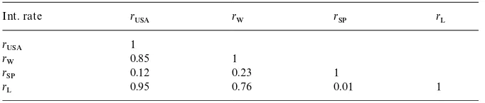
Table 1
Properties of the real interest rate measures (contemporaneous correlations)
Int. rate r
USA: U.S. T-Bill rate; W: weighted average rate of developed economies; SP: S&P 500 return; L: LIBOR rate. The T-Bill rate, the weighted rate, and the LIBOR rate are constructed using the IMF's International Financial Statistics (IFS). The S&P 500 return index is taken from the Ibbotson Associates Database. In constructing our ex ante real interest rates, we assume that in#ation follows a random walk. We use changes in the U.S. Consumer Price Index (CPI) as our measure of in#ation. The data are quarterly from 1963:1 to 1994:4.
Mendoza (1991), Schmitt-Grohe (1998), van Wincoop (1993), Beaudry and Guay (1996), and Barro and Sala-i-Martin (1990) use the U.S. and other countries'3-month T-bill rate. Schmitt-Grohe (1998) and Correia et al. (1992, 1995) use the S&P 500 index. Gagnon and Unferth (1995) use the Euro-market interest rates on certi"cates of deposit. Kose (1998) and Senhadji (1998) use the LIBOR rate. With respect to prices, van Wincoop (1993) and Barro and Sala-i-Martin (BSM) (1990) use the CPI, Beaudry and Guay (1996) use the GNP de#ator, and Schmitt-Grohe (1998) uses the GDP de#ator. For modeling in#ation expectations, the Livingston Survey, as well as many ARMA speci"cations have been employed.
T-Bill rates, have been employed as nominal interest rates. These di!erent
measures are not necessarily highly correlated with each other, as Table 1 shows for four ex ante real interest rates constructed from the same price index and
in#ation expectations, but with di!erent nominal interest rates. Half of the
correlations are less than 0.25. Second, as discussed extensively in Ingram et al. (IKS) (1994a,b, 1997) models in which the number of unobservable exogenous shocks is less than the number of observable endogenous variables imply that some of the observable variables are related deterministically. This feature exists in many small open economy models, and is fundamentally inconsistent with the data. The models are singular, which implies that it is not possible to back out a unique realization of unobservable exogenous shocks. In such models, there
are an in"nity of ways in which the importance of shocks*even orthogonal
shocks*in driving business cycles can be calculated. Finally, in any model with
multiple shocks, it is possible to determine the impact of any single shock only
by imposing often-arbitrary identi"cation restrictions. For example, one
often-imposed restriction in models of small open economies is that domestic shocks are uncorrelated with the world interest rate. Baxter and Crucini (1993, p. 432) "nd that this assumption is&empirically indefensible'. At best, then, only a range
of estimates * corresponding to di!erent identi"cation orderings of the
Our methodology draws from work by Ingram et al. (1994a, b), Hall (1986), Parkin (1988), and Lee (1996), among others. Ingram et al. (IKS) (1994a) back out exogenous shocks of a nonsingular closed economy real business cycle model to examine the importance of the productivity shocks. To study the cyclical behavior of home production IKS (1997) generate realizations of market and non-market hours. Using a similar methodology, Baxter and King (1998) back out the realizations of productivity and preference shocks, and Ambler and Paquet (1994) back out the time series of depreciation shocks. We follow Lee (1996) in our selection of the exogenous shocks and the unobservable endogenous variables, and in the method for backing out the exogenous shocks. Smith and Zin (1997) estimate the policy functions in a closed economy real business cycle model to generate realizations of output, consumption, and employment. There are other approaches to resolving the singularity problem. In order to ensure that the number of unobservable exogenous shocks equals the number of observable endogenous variables, measurement error can be added. See, for example, McGrattan (1994).
The purpose of this paper is to pursue an alternative quantitative methodo-logy to assess the importance of world real interest rates on small open economies. We continue to employ a standard dynamic stochastic small open economy model, (augmented to include preference and depreciation shocks). However, rather than parameterizing a shock process and using the model to solve for the endogenous variables, we let the model and the endogenous
variables tell us the exogenous shocks*including the world real interest rate*
that are consistent with the model. Speci"cally, we use the model's Euler
equations, data on the model's endogenous variables, as well as estimated
decision rules for the capital stock and net foreign assets, to recover the
exogenous shocks implied by the model and the data.Then, to compute the
importance of these backed-out shocks in driving business cycles, we perform variance decompositions. By altering the ordering of the shocks, we generate a range of estimates on the importance of each of the shocks.
To a large extent, then, our methodology reverses the standard approach.
Moreover, our approach deals with all three di$culties highlighted above. First,
we avoid the problems associated with calculating the appropriate world real interest rate; our backed-out interest rate measures are consistent with the model and the data. Second, because our model is nonsingular, we can evaluate the importance of the world real interest rate in business cycles without violating any relationships implied by the model. Third, by using shocks that are consis-tent with the model and by examining all possible orderings of shocks we do not need to take a particular stand on the relationship between them nor on their orthogonality.
We apply our methodology to quarterly Canadian data from 1961:1 to
1996:4. Our backed-out world real interest rate measure is quite di!erent from
proxies constructed from the data. Our variance decompositions indicate that
world real interest rate shocks can play a signi"cant role in explaining Canadian
business cycle#uctuations. If world interest rates shocks are ordered"rst, they
Mendoza (1991) was the"rst small open economy real business cycle model. See also Correia et al. (1992, 1995), Schmitt-Grohe (1998), Lee (1996), Sadka and Yi (1996), Kose (1998), and Senhadji (1998) for the use of dynamic small open economy models in evaluating the roles of di!erent shocks. Similar models have been used extensively in the literature on the intertemporal approach to current account behavior. See Baxter (1995) for a survey of dynamic general equilibrium business cycle models of open economies and their use in studying the sources and transmission of international business cycles.
Note that we use a constant discount factor, rather than the endogenous discount factor in Mendoza (1991) and Schmitt-Grohe (1998). Endogenous discount factors are used to ensure that models of small open economies have a stationary stochastic steady state. However, our approach does not require us to solve for the model's steady state or for the dynamics around the steady state. Moreover, because Correia et al. (1992, 1995) use a constant discount factor, the result that interest rates are not important is apparently robust to the type of discount factor. This latter inference is consistent with Kim and Kose (1999), who show that a model with a"xed discount factor generates similar business cycle implications to one with an endogenous discount factor.
cant fraction of variation in Canada's external balances: up to 62% (57%) of the
variation in net exports (net foreign assets) is explained by these shocks. These
quantitative"ndings contrast sharply with the results of Mendoza (1991) and
Schmitt-Grohe (1998). However, their results are qualitatively similar to our "ndings, and they are quantitatively similar to the variance decomposition results we obtain when real interest rates are ordered last.
The rest of this paper is organized as follows. In Section 2, we present our dynamic stochastic small open economy model. In Section 3, we calibrate the model to Canada and present our methodology on recovering the exogenous shocks. Our results are presented in Section 4, and Section 5 con-cludes.
2. The model
Our model is based on the standard small open economy real business cycle
model. The representative household maximizes expected lifetime utility
given by
R is consumption in periodt,lR is leisure,R is a time-varying preference
shock,is the consumption share parameter,is the discount factor, andis the
household's coe$cient of relative risk aversion.
The economy produces an internationally tradable good,y
R, according to
y
Our shocks are the same as those in Lee (1996). Stockman and Tesar (1995) employ preference shocks in a two-country business cycle model. Ambler and Paquet (1994) employ depreciation shocks in a closed economy real business cycle model. Greenwood et al. (1988) study a model where the marginal e$ciency of investment is a stochastic shock that is similar to the depreciation shocks we consider here. IKS state that&using a singular model when the variance-covariance matrix of the data is non-singular is equivalent to solving a set of inconsistent linear equations; there is no solution'. (IKS, 1994a, p. 416).
wherek
Ris the domestic capital stock at the beginning of the periodt,nR"1!lR
is labor hours,governs the share of income accruing to capital, andz
R is the
technology shock.
Following Baxter and Crucini (1993), we specify the following law of motion for capital:
R is investment,R is an exogenous depreciation shock, and())
repres-ents the standard adjustment cost function, with ())'0,())'0, and
())(0.
The representative household has access to world capital markets to borrow
and lend foreign"nancial assets. Net foreign assets,A
R, evolve according to:
A
R>"nxR#(1#rR)AR, (4)
wherenx
R is net exports measured in units of the domestic consumption good,
andr
R is the exogenously determined stochastic risk-free real interest rate from
periodt!1 tot. To prevent the representative household from playing a Ponzi
game, we impose the condition:
Finally, the aggregate resource constraint is
c
R#iR#nxR4yR. (6)
In our model there are four exogenous shocks, the world real interest rate and
a technology shock*which are the shocks in Mendoza's model*as well as
a preference shock and a depreciation shock. Because our model has four
observable endogenous variables, (consumption, investment, labor hours, and net exports) we need four exogenous shocks to insure that the model is non-singular. Singular models, that is, models with fewer exogenous unobservable variables than endogenous observable variables, imply deterministic relationships between the observable variables. These relationships are clearly violated in the data
We substitute (2) into (6), and substitute the resulting expression for net exports into (4). The representative household, then, maximizes
maxE
R and R are the LaGrange multipliers. The"rst-order conditions are
c
Eq. (11) governs the dynamics of net foreign assets. Eq. (12) equates the marginal rate of substitution between consumption and leisure to the marginal
product of labor. Eq. (13) is the intertemporal e$ciency condition pertaining to
3. Recovering the exogenous shocks
3.1. Parameter calibration
We calibrate our structural parameters to correspond to the existing real business cycle literature. Following Backus et al. (1992), the consumption share
parameter,, is set to 0.34, which is consistent with allocating, on average, 30%
of the endowment of non-sleeping time to labor market activities. The risk
aversion parameter,, is set to 1.5; this is an intermediate value between the
commonly used values of 2 and 1 (logarithmic utility). Following Mendoza (1991) and Schmitt-Grohe (1998), the share of capital income in the production,
, is set to 0.32. The discount factor and the initial value of the depreciation
shock are set to 0.988 and 0.025, respectively; both values are widely employed in real business cycle models calibrated to quarterly data (see, for example, King et al., 1988).
We specify the following functional form for the adjustment cost function:
equilibrium of the model is the same as that without adjustment costs. This
implies that (i/k)"i/k and (i/k)"1. In addition, (i/k) is set so that
the elasticity of the marginal adjustment cost function, "!(/)(i/k)\,
is equal to 15. This is the benchmark value used by Baxter and Crucini
(1993). Together, these three conditions determine the values of,, and.
We examine the sensitivity of our results to di!erent parameterizations in
Section 4.
3.2. Solving for the shocks
The standard real business cycle approach involves calibrating the model's
parameters, specifying forcing processes of the exogenous shocks, and then
solving the model. The model's solution would then be used to derive the"rst
and second moments of interest, calculate impulse responses, or compute variance decompositions. Our approach reverses this methodology: rather than produce simulated time series for endogenous variables, we use the observable endogenous variables and the orthogonality conditions implied by the Euler
equations to recover the exogenous shocks r
R,zR,R,R consistent with the
endogenous variables.
We treat consumption, investment, labor hours, and net exports as
observ-able; however, we treat the two endogenous state variables, k
While data on these two variables exist, we believe these data, because they are calculated as accumulated#ows, are poor counterparts to the concepts of capital and net foreign assets. In the case of capital, investment#ows are typically accumulated using depreciation rates that are assumed constant across di!erent types of capital and over time. Also, no valuation adjustments are typically made. In the case of net foreign assets, valuation adjustments are made, but di!erent adjustments produce di!erent numbers. According to the Bureau of Economic Analysis, depending on whether current cost valuation or market valuation is used, the U.S. net foreign asset (investment) position at yearend 1998 was!$1.2 trillion or!$1.5 trillion. Moreover, the net investment income from the U.S position was only about!$7 billion, which implies either that the$4.9 trillion in U.S. assets abroad were earning a considerably higher rate of return than the$6.2 trillion foreign assets in the US, or that the asset stocks were poorly measured.
We experimented with several policy functions to assess the sensitivity of our results to changes in functional forms. These changes have little e!ect on our main"ndings.
unobservable.To solve for these two variables, we estimate the policy functions
for capital and net foreign assets. We specify the following approximate policy
functionsk
As in Lee (1996), we choose approximate policy functions that are
computation-ally convenient and include most of the relevant state variables.The e!ect of
additional lagged variables is accounted for by the inclusion ofc
R. The exclusion
of the world real interest rate in the policy function for capital allows us to
estimateand sequentially, rather than simultaneously.
Replacingk
R>andAR>with our approximate policy functions, we estimate
the sample analogs of (13) and (11) given below:
1
In addition to Lee (1996), Smith and Zin (1997) and Beauchemin (1996) specify approximate policy functions and then estimate them by GMM.
K
is set by assuming the steady-state version of (3) and using data on investment.requals 1/!1 and
\is set to 0.025.Ais set by assuming the steady-state version of (4) holds for 1961:1. We truncate the"rst 8 data points from the recovered shocks so that the remaining part of the series is less sensitive to our choice of starting values.
In our model, there is no role for government expenditures. Hence, following Watson (1991), King et al. (1991), and Beaudry and Guay (1996), we exclude government expenditures from our measure of aggregate output.
The labor hours data is manufacturing hours worked per week, and is drawn from the OECD's Main Economic Indicators. The civilian employment data is drawn from the OECD Statistical Compendium on CD-ROM. This data is seasonally adjusted from 1965:1 to 1996:4. We impute the seasonally adjusted data for 1964:4 by multiplying the reciprocal of the 4-quarter growth rate from 1964:4 to 1965:4 of the non-seasonally adjusted employment level by the 1965:4 seasonally adjusted employment level, and similarly for 1964:3, 1964:2,2,1961:1.
lagged error terms from the estimation.
From the estimated policy functions, our model's equations, and initial values
k
,A,\, andr, we can recover the shocksrR,zR,R,R.Eq. (12) above
identi"es the series of preference shocks (R). To obtain the other shocks as well
as our estimates fork
Seasonally adjusted quarterly values of consumption, investment, and net
exports for Canada from 1961:1 to 1996:4 are drawn from the IMF's
Interna-tional Financial Statistics (IFS) naInterna-tional account series. Consumption is house-hold consumption expenditures; investment is the sum of gross capital
formation and inventory adjustments; net exports is the di!erence between
exports and imports of goods and services. Output,y
R, is the sum ofcR,iR and
nx
R.We convert these data to real per capita values by using the GDP de#ator
(1990 prices) from the IFS and population data drawn from the Bank of International Settlements database. Seasonally adjusted quarterly labor hours
and civilian employment data are drawn from the OECD.Following King
et al. (1988) total hours worked,n
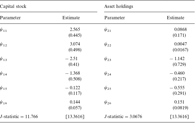
Table 2
Policy function coe$cients
Capital stock Asset holdings
Parameter Estimate Parameter Estimate
2.565 0.0868
(0.445) (0.171)
3.074 0.0047
(0.498) (0.0167)
!2.51 !1.142
(0.41) (0.729)
!1.368 !0.460
(0.508) (0.217)
!0.122 !0.555
(0.117) (0.291)
0.144 0.151
(0.057) (0.0819)
J-statistic"11.766 [13.3616] J-statistic"3.0676 [13.3616] The numbers in parentheses are the standard errors. TheJ-statistic is the chi-squared test statistic of the null hypothesis that the over-identifying restrictions (8 in each equation) hold. The numbers in brackets are the 10% signi"cance level critical values of the test.The policy functions are estimated on quarterly data from 1963:1 to 1996:4.
per week in the manufacturing sector and the employment rate normalized by the weekly time endowment.
4. Results
In this section, we"rst examine the properties of our backed out shocks. In so
doing, we provide some economic intuition on how our model works. We also compare our backed out interest rate series with measures constructed from the data. Finally, we examine the relative importance of our four exogenous shocks in inducing business cycles in Canada.
4.1. Properties of the exogenous shocks
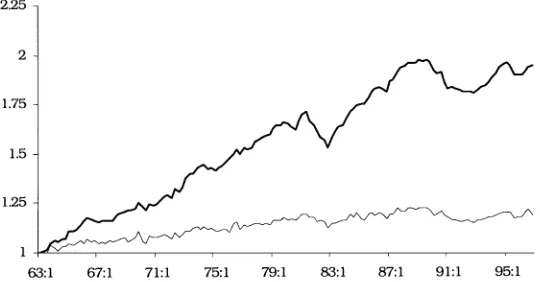
The coe$cients from estimating Eqs. (14) and (15) and their associated
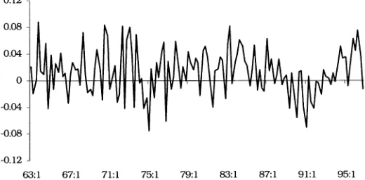
Fig. 1. Technology shocks and output. Quarterly technology shocks implied by the model (lighter line) and measured output (darker line) for each period from 1963:1 to 1996:4. Each series is normalized by its 1963:1 value.
Following the standard practice in the real business cycle literature, we detrend the series using Hodrick and Prescott (HP) (1997)"lter.
From Fig. 2, we see that the depreciation shocks are highly variable and occasionally negative. See Ambler and Paquet (1994) and Ingram et al. (1994a) for a discussion of occasionally negative depreciation and highly variable depreciation rates. They argue that a composite capital series represents many highly substitutable capital goods whose marginal productivities need not move together. Thus, there is substitution across capital types with"xed but di!ering depreciation rates and the composite depreciation rate can be highly variable.
over-identifying restrictions are satis"ed is not rejected at the 10% signi"cance
level.
Figs. 1}4 plot the four backed-out exogenous shocks and Table 3 presents
volatility and co-movement properties of these shocks.They show that the
world real interest rate is the most volatile of the four shocks, with a standard deviation 1.5 times larger than that of the depreciation shock and about 8 times
larger than that of the preference and technology shocks.Table 3 also shows
that the correlation coe$cient of the world real interest rate shock with the
technology shock and the depreciation shock is 0.38 and!0.32, respectively.
These correlations are consistent with the"ndings in Baxter and Crucini (1993).
In their two-country model calibrated to represent a large economy and a small
economy, they"nd that#uctuations in the world real interest rate are correlated
with domestic shocks.
Table 3
Properties of the estimated shocks (volatility and correlation) Variable Volatility Correlation with
r z
r 3.36 1.00
2.16 !0.32 1.00
0.47 !0.17 0.43 1.00
z 0.46 0.38 !0.65 !0.37 1.00
The technology (z) and preference () shocks are logged and then detrended by the Hodrick and Prescott (HP) (100)"lter. The world interest rate (r) and depreciation () shocks are measured in levels. Volatility is measured as the standard deviation of the (detrended) series.
Fig. 2. Depreciation shocks. Quarterly depreciation shocks implied by the model from 1963:1 to 1996:4.
Table 4
Correlation with macroeconomic variables
Correlation with r z
Output 0.24 !0.05 0.06 0.72
Consumption 0.07 !0.17 0.53 0.42
Investment !0.11 0.17 0.07 0.45
Net exports 0.52 !0.21 !0.38 0.11
Labor hours 0.05 0.48 0.61 0.11
The technology (z) and preference () shocks are logged and then detrended by the Hod-rick}Prescott (HP) (100)"lter.The world interest rate (r) and depreciation () shocks are measured in levels. All macroeconomic variables, except net exports, are logged and then HP(100)"ltered. Net exports is normalized by output, then HP(100)"ltered. The data range from 1963:1 to 1996:4.
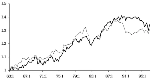
Fig. 4. Real interest rates. Quarterly real interest rates implied by the model from 1963:1 to 1996:4.
are positively correlated. This helps explain why a positive correlation between output and the world real interest rate shock can be generated. There is also a positive correlation (0.52) between the world real interest rate shock and net exports. All else equal, higher real interest rates imply more savings and less investment, leading to greater net exports. The technology shocks are not persistent; hence, the positive correlation between the world interest rate and technology shocks is probably not strong enough to induce changes in savings
and investment to completely o!set the direct e!ect of the higher interest rate.
Finally, the correlation between the real interest rate and consumption is positive largely because world interest rate shocks are positively correlated with domestic productivity shocks.
We examine the sensitivity of our results with respect to changes in the parameters of the model. In particular, we study whether the results in Tables 3
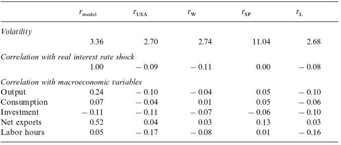
Table 5
Comparison of real interest rate shock with alternative interest rate measures
r
r31 r5 r1. r* <olatility
3.36 2.70 2.74 11.04 2.68
Correlation with real interest rate shock
1.00 !0.09 !0.11 0.00 !0.08
Correlation with macroeconomicvariables
Output 0.24 !0.10 !0.04 0.05 !0.10
Consumption 0.07 !0.04 0.01 0.05 !0.06
Investment !0.11 !0.11 !0.07 !0.06 !0.10
Net exports 0.52 0.04 0.03 0.13 0.03
Labor hours 0.05 !0.17 !0.08 0.01 !0.16
USA: U.S. T-Bill rate; W: weighted average rate of developed economies; SP: S&P 500 return; L: LIBOR rate.The U.S. T-Bill rate, the weighted rate, and the LIBOR rate are constructed using the IFS, and the S&P 500 return index is taken from the Ibbotson Associates Database. Consumption, investment, and net exports are drawn from the IFS; for the construction of the labor hours series, see fn. 13. All macroeconomic variables, except net exports and the interest rate measures, are logged and then HP(100)"ltered. Net exports is normalized by output, then HP(100)"ltered. The interest rate is measured in levels. The data range from 1963:1 to 1996:4.
This"nding is similar to"ndings in Beaudry and Guay (1996) and van Wincoop (1993).
the elasticity of the marginal adjustment cost, and the share of capital income in
total output. In general, we "nd our results to be quite robust. For example,
changes in the parameters do not a!ect the signs of the correlations between the
world real interest rate and output: interest rates are always weakly procyclical.
While changes in the parameters a!ect the volatility of the shocks, their e!ects
on the co-movement properties of the shocks are quite small.
It is worth comparing some of the properties of our interest rate measures with the properties of alternative measures. Table 5 presents comparisons involving the four ex ante interest rates presented in Table 1. While the volatility of our interest rate measure is similar to the other measures, there is very little
correlation between the other measures and our measure.Also, the alternative
interest rate measures tend to be negatively correlated with output, but our
model-generated interest rate is positively correlated with output. This"nding is
the same as in the Beaudry and Guay (1996) closed economy framework. However, the correlations with net exports and investment tend to be broadly
similar across the di!erent interest rate measures. Summarizing, our interest rate
shock di!ers from the alternative measures on two important dimensions, but
See Ingram et al. (1994a, b), Cochrane (1994) and King (1995) for extensive discussions of the standard approach and its shortcomings. IKS (1994a), for example, forcefully argue that there is no way to get a de"nitive answer to the question of how much variation in output can be attributed to technology shocks. Our variance decomposition method is closely related to those employed in Ingram et al. (1994a), McGrattan (1994), Kouparitsas (1997), and Kose (1998).
Our approach employs the familiar Choleski decomposition. It is possible of course to perform other decompositions, such as those employed in Clarida and Gali (1994) and other papers. However, the identi"cation restrictions in these papers typically involve linkages between nominal and real variables, i.e., money shocks have no e!ect on output. Our setting involves only real shocks, and it is di$cult to think of intuitive restrictions that would involve a shock having zero e!ect on one of our variables. Hence, we focus on the more traditional triangular decompositions. Pesaran and Shin (1998) and others have developed `generalizeda variance decompositions, in which orthogonalized shocks are not required. However, one drawback of this approach is that the variance decompositions do not add up to 1.
4.2. Importance of shocks in business cycleyuctuations
In a multi-shock model, measuring the contribution of any single shock to
business cycle #uctuations is di$cult because the shocks are correlated with
each other, as we have shown for Canada. The standard approach in the RBC literature, which examines each shock in isolation from the other shocks, can then yield misleading inferences. Our approach is to apply a variance decompo-sition method analogous to what is employed in the vector autoregression
(VAR) literature. Following the usual VAR setting, we perform variance
decompositions in our framework by imposing a recursive ordering scheme that
generates orthogonal shocks from the correlated shocks.Because the order of
precedence of the shocks is crucial to determining the shocks'relative
import-ance in explaining the variimport-ance of a particular macroeconomic variable, and because we have little prior information on which ordering to employ, we compute the contribution of each shock for all possible orderings (24).
To illustrate, let [r
R,zR,IR,R],t"1,¹, denote the vector of time series of our
four shocks. The ordering [r
R,zR,IR,R] indicates that the real interest rate is"rst
in precedence } any contemporaneous correlation between r
R and the other
shocks is&assigned'tor
R *and the preference shock is last*only that part of
Runcorrelated with the other shocks is&assigned'toR. We obtain the variance
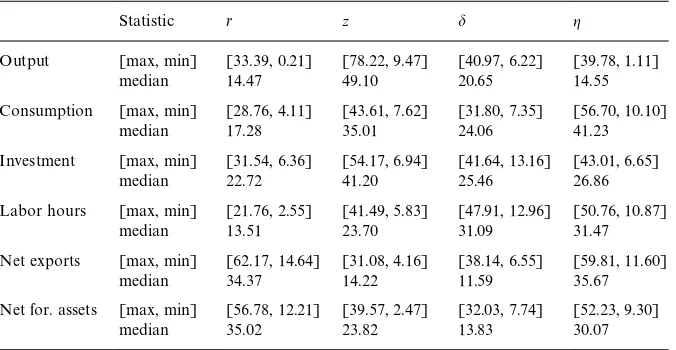
Table 6
Variance decompositions
Statistic r z
Output [max, min] [33.39, 0.21] [78.22, 9.47] [40.97, 6.22] [39.78, 1.11]
median 14.47 49.10 20.65 14.55
Consumption [max, min] [28.76, 4.11] [43.61, 7.62] [31.80, 7.35] [56.70, 10.10]
median 17.28 35.01 24.06 41.23
Investment [max, min] [31.54, 6.36] [54.17, 6.94] [41.64, 13.16] [43.01, 6.65]
median 22.72 41.20 25.46 26.86
Labor hours [max, min] [21.76, 2.55] [41.49, 5.83] [47.91, 12.96] [50.76, 10.87]
median 13.51 23.70 31.09 31.47
Net exports [max, min] [62.17, 14.64] [31.08, 4.16] [38.14, 6.55] [59.81, 11.60]
median 34.37 14.22 11.59 35.67
Net for. assets [max, min] [56.78, 12.21] [39.57, 2.47] [32.03, 7.74] [52.23, 9.30]
median 35.02 23.82 13.83 30.07
In each cell, the share of the variable's variance explained by a particular shock is reported.&max',
&min', and&median'refer to the upper bound, lower bound, and median of the variance decomposi-tions across all orderings. The technology (z) and preference () shocks are"rst logged and then detrended by the Hodrick and Prescott (HP) (100)"lter. The world interest rate (r) and depreciation () shocks are in levels. Consumption, investment, and net exports are drawn from the IFS, and the labor hours series is taken from the OECD Main Economic Indicators. All macroeconomic variables, except net exports and net foreign assets, are logged and then HP(100)"ltered. Net exports and net foreign assets are normalized by output, then HP (100)"ltered. The data range from 1963:1 to 1996:4.
respectively. As¸ becomes very large, the variance of
R, var(R), goes to zero,
because current and lagged values of the four shocks account for all of the
variation in output#uctuations. For each regression we set the lag length at the
smallest number for which var(
R)(0.01 var(yR). The fraction of the variance of
output explained by each shock is then given by:
qX"var(yXR)
Hence, the sum of the contributions of the shocks is one. We follow this
procedure for all twenty-four orderings, and then repeat it for "ve other
that for each variable and each shock, the range of variances is large, indicating a good deal of sensitivity to the ordering assumptions. For example, technology shocks explain as much as 78% of output variation, which occurs when it
is ordered"rst, and as little as 9.5% of output variation, which occurs when it
is ordered last.
The third column of the table suggests that interest rate shocks exert their
largest e!ect on net exports and net foreign assets, and can account for over 50%
of the #uctuations in these variables. The median variance attributable to
interest rates was about 35% for these two variables. The medians also indicate that interest rate shocks accounted for more variation in net foreign assets than the other shocks, and they accounted for more variation in net exports than all but the preference shock. Even when interest rates are ordered last, they still explain over 12% of the variation in net exports and net foreign assets. The table
also shows that interest rate shocks can account for up to 22}33% of the
#uctuations in output, investment, consumption, and labor hours. The median
variance attributable to interest rates is about 14}23% for these four variables.
Examining the impact of the other shocks, we see that our results suggest that
technology shocks tend to explain the lion's share of output and investment
variation, and preference shocks tend to explain more consumption variation than do the other shocks. Depreciation shocks have their greatest impact on
investment and labor hours. Our"ndings on the importance of depreciation and
preference shocks mirror results in Ambler and Paquet (1994) and Stockman
and Tesar (1995), who "nd that introducing depreciation (preference) shocks
into a one-country (two-country) real business cycle model, respectively,
im-proves the"t of the model to the data.
Our main results are not too sensitive to departures from the benchmark
parameterization. For example, as the risk aversion coe$cient increases from
1.5 to 5, the percentage of output variance explained by the world real interest rate shock decreases. The drop occurs because the volatility of the backed-out interest rate shock declines. Changes in the elasticity of the adjustment cost and of the share of capital income in total income also do not have any major impact in the results. The contribution of the real interest rate to explaining net exports and net foreign assets exhibits similar ranges as those listed in Table 6.
At this point it is instructive to compare our results to those of Mendoza
(1991), Schmitt-Grohe (1998) and Correia et al. (CNR, 1995)*especially the
two former studies, because they were also based on Canadian data. We"nd
that the world real interest rate shock can account for up to 33%, 57% and 62% of output, net foreign asset, and trade balance variation in Canada. By contrast,
Mendoza (1991, p. 809)"nds that interest rate shocks have only&minimal'e!ects
on model variables. Schmitt-Grohe (1998) uses impulse responses to assess the importance of interest rate shocks (driven by changes in U.S. output) to Canada. She"nds that the interest rate transmission mechanism alone cannot generate
addition, CNR conclude that interest rate shocks exert small e!ects on output, consumption, and hours worked. Hence, our results clearly suggest a much stronger role than previous studies for interest rate shocks in generating
macro-economic#uctuations in small open economies.
Because our methodology is considerably di!erent from their methodologies,
there could be many reasons why our results could di!er from theirs. Our
estimated interest rate measure is quite di!erent from the proxies that their
shock processes are characterized from. We allow for more shocks than just interest rate and technology shocks. In addition, we do not take a stand on the relation between the shocks or on the orthogonality of the shocks. Nevertheless, we implement a sensitivity analysis to assess whether the way we generate our interest rate shocks or the way we calculate the contribution of these shocks to macroeconomic volatility is more important in driving our results. We engage in the same variance decomposition exercises, but we replace our interest rate measure with alternative interest rate measures, including the U.S. T-Bill rate,
the S&P 500 return, and a weighted average of several developed countries'
interest rates. We use the same backed out preference, depreciation, and
produc-tivity shocks as in the original exercises. We"nd that the contribution of interest
rates to explaining macroeconomic volatility decreases. For example, the me-dian contribution of interest rates to the volatility of net exports and of foreign assets is about 15%, compared to about 35% in the original decompositions. However, the median contribution of interest rates to output and consumption volatility decreases only slightly, to 12% from 14% (output) and to 16% from 17% (consumption). If the contribution of interest rates had fallen to zero, this would have suggested that the way we generate the interest rate shocks is important and the results are not driven by our multiple-ordering variance decompositions. If the contribution of interest rates had remained unchanged, this would have suggested that our variance decompositions are important and
the results are not driven by the way we generated the shocks. Our"ndings are
between these two extremes, suggesting that our main results are due toboth
features of our methodology * the backed-out shocks and the
multiple-ordering variance decompositions.
Despite the di!erences in methodology, however, there are several similarities
in the results. The benchmark model in Mendoza (1991) involves only techno-logy shocks. When interest rate shocks are added, the contribution to
macroeco-nomic#uctuations is quite small. For example, the standard deviation of output
rises from 2.81% to 2.84%. This is consistent with our results when interest rate
shocks are ordered last. We"nd that they account for only 0.21% of output
#uctuations, and less than 7% of the#uctuations in consumption, hours, and
investment. From impulse responses, CNR"nd that, compared to technology
shocks, interest rate shocks exert a relatively larger e!ect on net exports and
a relatively smaller e!ect on output. From our variance decompositions, we
There is one additional similarity between Mendoza (1991) and our results. Mendoza's Table 5 shows that even when the correlation between technology shocks and interest rate shocks is$0.9, the moment properties of key variables are basically unchanged. We note that when the shocks are this highly correlated, variance decompositions that order interest rates"rst (second) will tend to attribute much (little) of the variation in output and other variables to interest rates.
tion of interest rate shocks to the volatility of output is about 15%, its median contribution to the volatility of net exports is about 35%. Finally, Mendoza
(1991)"nds that, as the standard deviation of interest rate shocks increases to
about "ve times the standard deviation of technology shocks, #uctuations in
output and investment also increase. The standard deviation of our interest rate shock is an even larger multiple of the standard deviation of our technology shock. We surmise this helps increase the fraction of output and investment
#uctuations attributable to interest rates.
Summarizing, we"nd that interest rate shockscanbe important in explaining
#uctuations * particularly #uctuations in net exports and net foreign assets
*in a small open economy. This is in contrast to the results of several recent
quantitative studies on this topic. However, our results arequalitativelysimilar
to these results, indicating the presence of similar economic mechanisms at
work. Also, our results become quantitatively similar to their results when
interest rate shocks are ordered last in our variance decompositions.
5. Conclusion
Most models of small open economies posit several channels by which world shocks are transmitted to the small economy. Of these channels, the interest rate channel is often given special prominence. Hence, it is surprising that several recent quantitative analyses applying the standard real business cycle approach
have found that#uctuations in world interest rates have little e!ect on domestic
investment, output, net exports, and net foreign assets. In this paper we employ an alternative approach to quantitatively address the importance of interest rate shocks in a small open economy. The key point of departure is that we use the model and data on the endogenous variables to back out the exogenous shocks that are consistent with the model, while the standard approach posits statistical processes for the exogenous shocks (based on proxies of these shocks) and feeds these processes through the model to generate the endogenous variables that are
consistent with the model. We view our approach as addressing di$culties in the
We apply our approach to Canada, a country that has been studied quite
thoroughly via the standard approach. Our"ndings indicate that world interest
rate shocks can have large e!ects, particularly on net exports and net foreign
assets, but also on output. Our sensitivity analysis indicates that both features of
our methodology*the backed-out shocks and the multiple-ordering variance
decompositions* are driving our"ndings. We conclude that the world real
interest rate can be an important transmission mechanism of world business cycles to small open economies. Nevertheless, the results of the other recent research are qualitatively similar to our results, and quantitatively similar to the lower bound of our variance decompositions, occurring when the world real interest rate is ordered last.
In our model, we do not include"scal and monetary policy shocks, which are
important in understanding business cycle dynamics in open economies. It would be useful to apply this methodology to examine the role of these shocks in a more complex small open economy model.
6. For further reading
The following references are also of interest to the reader: Hansen, 1982; Hercowitz, 1986; Ingram, 1995; Prescott, 1986.
References
Ambler, S., Paquet, A., 1994. Stochastic depreciation and the business cycle. International Economic Review 35 (1), 101}116.
Backus, D.K., Kehoe, P.J., Kydland, F.E., 1992. Real business cycles. Journal of Political Economy 100, 745}775.
Barro, R., Sala-i-Martin, X., 1990. World real interest rates. NBER Macroeconomics Annual 1990 15}61.
Baxter, M., 1995. International trade and business cycles. In: Gene Grossman, Kenneth Rogo!, (Eds.), Handbook of International Economics. North-Holland, Amsterdam.
Baxter, M., Crucini, M., 1993. Explaining saving-investment correlations. American Economic Review 83, 416}436.
Baxter, M., King, R., 1998. Productive externalities and business cycles. European Economic Review, forthcoming.
Beauchemin, K.R., 1996. Whither the stock of public capital? Working paper, University of Colorado at Boulder.
Beaudry, P., Guay, A., 1996. What do interest rates reveal about the functioning of real business cycle models? Journal of Economic Dynamics and Control 20, 1661}1682.
Clarida, R., Gali, J., 1994. Sources of real exchange rate#uctuations: How important are nominal shocks? Carnegie-Rochester Conference Series on Public Policy 41, 1}56.
Cochrane, J.H., 1994. Shocks. Carnegie Rochester Conference Series on Public Policy 41, 295}364.
Correia, I., Neves, J.C., Rebelo, S., 1995. Business cycles in a small open economy. European Economic Review 39, 1089}1113.
Gagnon, J.E., Unferth, M.D., 1995. Is there a world real interest rate? Journal of International Money and Finance 14, 845}855.
Greenwood, J., Hercowitz, Z., Hu!man, G., 1988. Investment, capacity utilization and the real business cycle. American Economic Review 78, 402}416.
Hall, R.E., 1986. The role of consumption in economic#uctuations. In: Gordon, R.J. (Ed.), The American business cycle: continuity and change. University of Chicago Press, Chicago, pp. 237}266.
Hansen, L., 1982. Large sample properties of generalized method of moment estimation. Econo-metrica 50, 1029}1054.
Hercowitz, Z., 1986. The real interest rate and aggregate supply. Journal of Monetary Economics 18, 121}145.
Hodrick, R.J., Prescott, E.C., 1997. Postwar U.S. business cycles: an empirical investigation. Journal of Money, Credit, and Banking 29, 1}16.
Ingram, B., 1995. Recent advances in solving and estimating dynamic, stochastic macroeconomic models. In: Hoover, K. (Ed.), Macroeconometric Developments, Tensions and Prospects. Kluwer Academic Publishers, Dordrecht, pp. 15}47.
Ingram, B., Kocherlakota, N., Savin, N.E., 1994a. Explaining business cycles: A multiple shock approach. Journal of Monetary Economics 34, 415}428.
Ingram, B., Kocherlakota, N., Savin, N.E., 1994b. Rational expectations shock estimation. Mimeo, University of Iowa.
Ingram, B., Kocherlakota, N., Savin, N.E., 1997. Using theory for measurement: An analysis of the cyclical behavior of home production. Journal of Monetary Economics 40, 435}456. Kim, S.H., Kose, M.A., 1999. Dynamics of open economy business cycle models:&understanding the
role of the discount factor'. Manuscript, Brandeis University.
King, R.G., 1995. Quantitative theory and econometrics. Federal Reserve Bank of Richmond Economic Quarterly 81, 53}105.
King, R.G., Plosser, C.I., Rebelo, S., 1988. Production, growth, and business cycles I: The basic neoclassical model. Journal of Monetary Economics 21, 195}232.
King, R.G., Plosser, C.I., Stock, J.H., Watson, M.W., 1991. Stochastic trends and economic
#uctuations. American Economic Review 81, 819}840.
Kose, M.A., 1998. Explaining business cycles in small open economies. Working paper, Brandeis University.
Kouparitsas, M., 1997. North-South business cycles. Working paper, Federal Reserve Bank of Chicago.
Lee, J.S., 1996. Change of cyclical pattern in developing countries: evidence from Korea. Working paper, The Bank of Korea.
McGrattan, E.R., 1994. The macroeconomic e!ects of distortionary taxation. Journal of Monetary Economics 33, 573}601.
Mendoza, E.G., 1991. Real business cycles in a small open economy. American Economic Review 81, 797}889.
Obstfeld, M., Rogo!, K., 1995. The intertemporal approach to the current account. In: Gene Grossman, Kenneth Rogo!, (Eds.), Handbook of International Economics. North-Holland, Amsterdam.
Parkin, M., 1988. A method for determining whether parameters in aggregative models are structural. Carnegie-Rochester Conference Series on Public Policy 29, 215}252.
Pesaran, M.H., Shin, Y., 1998. Generalized impulse response analysis in linear multivariate models. Economics Letters 58, 17}29.
Sadka, J.C., Yi, K. 1996. Consumer durables, permanent terms of trade shocks, and the recent U.S. trade de"cits. Journal of International Money and Finance 15, 797}811.
Schmitt-GroheH, S., 1998. The international transmission of economic#uctuations. Journal Interna-tional Economics 44, 257}287.
Senhadji, A., 1998. Dynamics of the trade balance and the terms-of-trade in LDCs: the S-curve. Journal of International Economics 46, 105}131.
Smith, G.W., Zin, S.E., 1997. Real business cycle realizations. Carnegie-Rochester Series on Public Policy 47, 243}280.
Stockman, A., Tesar, L., 1995. Tastes and technology in a two-country model of the business cycle: explaining international comovements. American Economic Review 85, 168}185.
van Wincoop, E., 1993. Real interest rates in a global bond economy. Working Paper no. 52, Innocenzo Gasparini Institute for Economic Research.