www.elsevier.nl/locate/cam
On the numerical solution of direct and inverse problems
for the heat equation in a semi-innite region
Roman Chapko
Department of Applied Mathematics and Computer Science, Lviv University, 290602 Lviv, Ukraine
Received 6 May 1998; received in revised form 2 April 1999
Abstract
We consider the initial boundary value problem for the heat equation in a region with innite and nite boundaries (direct problem) and the related problem to reconstruct the nite boundary from Cauchy data on the innite boundary (inverse problem). The numerical solution of the direct problem is realized by a boundary integral equation method. For an approximate solution of the inverse problem we use a regularized Newton method based on numerical approach for the direct problem. Numerical examples illustrating our results are presented. c1999 Elsevier Science B.V. All rights reserved.
Keywords:Heat equation; Semi-innite region; Initial boundary value problem; Inverse boundary problem; Green’s function; Integral equation; Collocation method; Trigonometric interpolation; Newton method; Regularization
1. Introduction
The numerical solution of the initial boundary value problems for the linear parabolic equation is of considerable signicance for a number of applied sciences [11]. These problems are of partic-ular interest for the case of unbounded domains. Then almost all numerical methods are based on boundary integral equations [3,4,7,13,20]. Since the unknown solution has to be found according to the known boundary and boundary data, these linear problems are referred to as the direct problems. The inverse problems for a parabolic equation can be divided into the following principal groups [21]: (1) the problems of the estimation of the heat ux history along a boundary part of a domain from a known temperature measurements on the rest of the boundary and at interior locations; (2) the problems of determining the initial condition if the temperature distributions inside a domain are known at some time; (3) the problems on recovering the diusion coecient from boundary
E-mail address: [email protected] (R. Chapko)
measurements of the solution of a parabolic equation; (4) the problems in determining a boundary part for the bounded domain from a knowledge of the rest of the boundary, the heat and the heat ux on it (see [1,2,5,8]).
In this paper we consider the direct and the related inverse problems from the fourth group for the heat equation in the case of a specic unbounded domain. Primarily we are interested in the aspects of the numerical solution of these problems.
Let D2:={x∈R2:x2¿0} be the upper half-plane in R2 and D1 a simply connected bounded
domain in R2 with the boundary
1 of the class C2 such that D1⊂D2. Let T ¿0, I:= (0; T], 2:={x:x2 = 0; ∞¡ x1¡∞}; D:=D2\D1 and let ’ be a given function on @D×I. Further
denote by ’1 and ’2 the restrictions of ’ on 1×I and 2 ×I, respectively. We shall consider
the following direct initial boundary value problem for the heat equation: Find a bounded function u(x; t) satisfying
@u
@t = u in D×I; (1.1)
u(·;0) = 0 inD; (1.2)
u=’ on @D×I: (1.3)
We shall also consider the following related inverse boundary value problem. Under the assumption that ’1= 0, ’2 6= 0, to determine the boundary 1 from a knowledge of the heat ux
@u
@(x; t) on ;
where :={x:x2= 0; 06x161} ×[T0; T1], [0; 1]⊂(−∞;∞) with0¡ 1, [T0; T1]⊆[0; T] with
T0¡ T1 and is the outward unit normal on 2. The existence and uniqueness of classical or weak
solutions for the initial boundary value problem (1.1) – (1.3) are well established [12,18]. For our inverse problem analogous to [8] we have the following uniqueness result.
Theorem 1.1. LetD1;1 andD1;2 be two bounded domains in the upper half-plane with the bound-aries 1;1 and 1;2; respectively. Let u1 and u2 be the classical solutions to the initial boundary value problems (1:1) – (1:3) in the domains D2\D1;1 and D2\D1;2; respectively; for ’1= 0 and
’26= 0. Let us assume that the heat uxes of both solutions coincide:
@u1=@=@u2=@ on :
Then 1;1= 1;2.
The outline of the paper is as follows. In Section 2 we will describe the numerical solution of the initial boundary value problem (1.1) – (1.3) via boundary integral equations of the rst kind. For the integral representation of the solution we use the single-layer potential with the Green’s function for the half-plane. Some aspects of using the Newton method for the numerical solution of our inverse problem are described in Section 3. Finally, in Section 4, we present the results of some numerical experiments.
2. Numerical solution of the direct problem
The special features of the domain Ddetermine the numerical method for the solution of the direct problem (1.1) – (1.3). Since D is an unbounded domain, clearly most ecient numerical method is the application of boundary integral equations. To avoid the determination of a density on the innite boundary we use the single-layer approach with a Green’s function as a special fundamental solution. The Green’s function for the heat equation in the upper half-plane has the form
G∞(x−y; t) :=G(x1−y1; x2−y2; t)−G(x1−y1; x2+y2; t);
where
G(x1; x2; t) =
e−|x2 1+x
2 2|
2=4t
t ; t ¿0; x
2
1+x22¿0 (2.1)
is the fundamental solution of the heat equation inR2. Then we can seek the solution of the problem
(1.1) – (1.3) in the form
u(x; t) = 1 4
Z t
0
Z
1
q(y; )G∞(x−y; t−)ds(y) d
−41
Z t
0
Z
2
’2(y; )
@G∞
@(y)(x−y; t−)ds(y) d; (x; t)∈D×I; (2.2)
with a density q on 1×I and the outward unit normal on 2. The heat potential (2.2) satises
the heat equation (1.1), the homogeneous initial condition (1.2) and the boundary condition on the innite curve 2. By the classical results on the continuity of the single-layer potential [12] and by
the properties of Green’s functions [14] the problem (1.1) – (1.3) is reduced to the integral equation of the rst kind:
1 4
Z t
0
Z
1
q(y; )G∞(x−y; t−) ds(y)d=f(x; t); (x; t)∈ 1×I; (2.3)
where
f(x; t) =’1(x; t) +
1 4
Z t
0
Z
2
’2(y; )
@G∞
Theorem 2.1. For any given function’1∈H 1=2;1=4
00 ( 1×I) and’2∈L2( 2×I)the integral equation
(2:3) possesses a unique solution q∈H00−1=2;−1=4( 1×I).
We assume that the boundary curve is given through a parametric representation
1={x(s) = (x1(s); x2(s)): 06s62};
where x:R→R2 is twice continuously dierentiable and 2-periodic with |x′(s)|¿0 and x
2(s)¿0
for all s. Then we transform (2.3) and(2.4) into the parametric form
1 4
Z t
0
Z 2
0
(; )K(1)(s; ;t; ) dd=F(s; t); (s; t)
∈[0;2]×I (2.5)
and
F(s; t) = 2g1(s; t) +
1 2
Z t
0
Z ∞
−∞
g2(; )K(2)(s; ;t; ) dd; (2.6)
where we have set (s; t) :=q(x(s); t)|x′(s)
|, g1(s; t) :=’1(x(s); t), and g2(s; t) := ’2(s;0; t), and
where the kernels are given by
K(1)(s; ;t; ) :=G∞(x(s)−x(); t−) and
K(2)(s; ;t; ) := − x2(s) (t−)2exp
(
−(x1(s)−)
2+x2 2(s)
4(t−)
)
for s 6= . For the semi-discretization of the integral equation (2.5) we use a collocation method with respect to the time-variable [3,4,20]. We choose an equidistant mesh on I by
tn=nht; n= 0; : : : ; N; ht=T=N;
and use the constant-time interpolation for the unknown density and for the given boundary function g2. Then for t=tn from (2.5) and (2.6) we obtain for approximations n(s)≈(s; tn) the
following system of Fredholm integral equations of the rst kind:
1 2
Z 2
0
n()K0(1)(x(s); ) d=Fn(s)−
1 2
n−1
X
m=1
Z 2
0
m()Kn(1)−m(x(s); ) d (2.7)
for s∈[0;2]; n= 1; : : : ; N: Here we have set
Fn(s) = 2g1; n(s)−
1 2
n
X
m=1
Z ∞
−∞
g2; m()K (2)
n−m(x(s); ) d; (2.8)
where gi; n(s) :=gi(s; tn), i= 1;2; and where the functions Kp(i) are given by
Kn(i−)m(x(s); ) :=
Z tm
tm−1
Ki(s; ;tn; ) d:
After some elementary calculations we nd
K(1)
p (x(s); ) =K (1)
1; p(x(s); )−K (1)
where have to be set equal to zero). Here we introduced the functions
r1(x(s); ) :=|x(s)−x()|; r2(x(s); ) := ([x1(s)−x1()]2+ [x2(s) +x2()]2)1=2
and
˜
r(x(s); ) := ([x1(s)−]2+x22(s)) 1=2;
and E1 denotes the exponential integral function (see [19]). Since the function E1 has the expansion
E1(z) =−−lnz−
Thus we have to solve a system of integral equations of the rst kind with a logarithmic singu-larity. For a full discretization of this system we combine a quadrature method and a collocation method based on trigonometric interpolation. For this we choose an equidistant mesh by setting
sj:=j=M; j= 0; : : : ;2M−1;
and use the following two quadrature rules:
with the weights
For the numerical calculation of the integrals on an innite interval in (2.8) we use the quadrature rule
These quadrature formulas are obtained by replacingg by its trigonometric interpolation polynomial in the case of (2.10) and (2.11) (see [16]) and by sinc approximation in the case of (2.12) (see [22]) and then integrating exactly. For the rules (2.10) and(2.11) in the case of periodic analytic functions g and for the rule (2.12) in the case of analytic functions g satisfying g(s) = O(e−|s|) for
|s| → ∞ and some positive constant we obtain exponential convergence.
Now we apply the quadrature rules (2.10) and (2.11) in the integral equations (2.7) and the rule (2.12) in (2.8) and then discretize the corresponding approximate equations by a trigonometric collocation. As a result we obtain a sequence of linear systems
2M−1 integral equation of the type (2.7) in [6] in a Holder space and in [17] in a Sobolev space setting. In the case of an analytic boundary and boundary data as shown by the error analysis in [6,17], we obtain the exponential convergence for the numerical solution of the integral equations (2.7) with respect to the number M of the space discretization. The numerical experiments (see Section 4) conrm this and show also the linear convergence with respect to the number N of the time discretization for the used numerical method.
For the numerical implementation of the inverse problem we need the approximations for the normal derivative of the solution (2.2) on the boundaries. From the jump relations for the normal derivative of a single-layer potential [12] and from the continuity for the normal derivative of a double-layer potential [10,15] we have
@u
Then connecting formula (2.15) with the numerical solution of integral equation (2.3) we have the following approximation for the ux on 1:
for p= 0; : : : ; N −1 (for p= 0 the second terms on the right-hand sides have to be set equal to
i;0 have a pronounced delta function
like behavior. A similar problem is arising also in another numerical method for the parabolic problems [7,20]. For the numerical experiments in Section 4 we choose the time discretization parameter not very large and co-ordinated it with the spatial discretization parameter, i.e. we increase the number M of quadrature points when the number N of collocation points with respect to the time is increased. This reects the general requirement to balance spatial and time discretization in the numerical solution of the nonstationry problems.
The numerical calculation of the ux (2.16) causes additional diculties because of a strong singularity in the kernel of the second term. We shall consider this case in more detail. Let
P(x; t) := 1 After the parametrization of 2 and the constant-time interpolation for ’2 we have
P(s; tn)≈
we consider only the integral with the integrand H0(2)(s; ) as a nite part integral, that is, as Hadamard’s hypersingular integral. By partial integration we obtain
Here the rst integral is considered as a Cauchy singular integral. For the numerical integration of this integral we use the sinc quadrature rule [22]
1
Thus, nally, the approximate heat ux on 2 is given by
@u
3. The numerical solution of the inverse problem
The solution of the direct initial boundary value problem (1.1) – (1.3) denes a nonlinear operator
F: 1 → @u
@(x; t); (x; t)∈;
which maps the curve 1 onto the ux@u=@ on the line 2. In this sense the solution of our inverse
problem consists in the solution of the nonlinear equation
F( 1) = ; (3.1)
where (x; t) :=@u=@(x; t); (x; t)∈: Let us assume that 1 is starlike, i.e.
x(s) = (r(s)coss; r(s)sins+d); 06s62 (3.2)
with a positive functionr(s)∈C2(
1) and a positive constantd, such thatx2(s)¿0 for alls. Clearly
r(s) is to be found. We transform Eq. (3.1) into the parametric form
F(r) =(s; t); (s; t)∈∗; (3.3)
where (s; t) := (s;0; t) and ∗:= [
Assume that the curve ˜1, with the parametric representation z(s) is an approximation for the
curve 1 and leth(s) be the unknown correction such that ˜z(s) =z(s) +h(s) is a new approximation.
We look for h(s) in the form
h(s) = (q(s)coss; q(s)sins+d); (3.4)
where q(s) is the unknown. After the linearization of Eq. (3.3) we get the following approximating linear equation with respect to h(s):
F(r) +F′(r;h) =(s; t); (s; t)∈∗: (3.5)
We approximate q(s) in the form
q(s) =
K
X
j=1
ajqj(s) (3.6)
with basis functions qj(s). The collocation method for (3.5) with respect to the collocation points
( ˜sk;t˜i)∈∗, k= 1; : : : ; Minv, i= 1; : : : ; Ninv, yields the system of linear equations K
X
j=1
ajF′(r;hj)( ˜sk;t˜i) =( ˜sk;t˜i)−F(r)( ˜sk;t˜i); (3.7)
where hj(s) := (qj(s)coss; qj(s)sins+d) and MinvNinv¿ K. Analogous to the case of the inverse
problems for the heat equation in a bounded domain [8] for the derivative F′(r; h) we have the following result:
Theorem 3.1. LetD˜1 be a bounded domain with the boundary ˜1 andD˜:=D2\D˜1.Let’2∈L2( 2×
I); h∈C2( ˜
1;R2) andu be a weak solution of the initial boundary value problem (1:1) – (1:3) in
˜
D×I with ’1= 0. Then the domain derivative F′(r;h) exists and is given by
F′(r;h) = @u
′
@
;
where u′ solves the heat equation @u′
@t = u
′ in ˜D
×I (3.8)
in the weak sense and satises the boundary condition
u′=−h·@u
@ on ˜1×I and u
′= 0 on
2×I: (3.9)
Here is the outward unit normal on ˜1.
Due to the linear equation (3.5) being an ill-posed equation, we have to incorporate some regu-larization to stabilize our problem, for example a Tikhonov reguregu-larization. Hence, we replace (3.7) by the following least-squares problem to minimize the penalized residual
T:=
K
X
k=1
wka2k+ Minv
X
i=1 Ninv
X
j=1
K
X
k=1
akF′(r;hk)( ˜si;t˜j)−( ˜si;t˜j) +F(r)( ˜si;t˜j)
with some regularization parameter ¿0 and some positive weights w1; : : : ; wK. Minimizing of T
with respect to a1; : : : ; aK is equivalent to solving the following linear system:
wpap+ K
X
k=1
ak Minv
X
i=1 Ninv
X
j=1
F′(r;hk)( ˜si;t˜j)F′(r;hp)( ˜si;t˜j)
=
Minv
X
i=1 Ninv
X
j=1
{( ˜si;t˜j)−F(r)( ˜si;t˜j)}F′(r;hp)( ˜si;t˜j); p= 1; : : : ; K: (3.10)
We choose the weights wp as in the Levenberg–Marquardt algorithm:
wp= Minv
X
i=1 Ninv
X
j=1
F′(r;qp)( ˜si;t˜j)F′(r;qp)( ˜si;t˜j); p= 1; : : : ; K:
Finally, we summarize the description of one step of the Newton method as follows:
1. Given the initial approximation z0 for 1 (the circle as an example), solve the direct problem
(1.1) – (1.3) by the method in Section 2 and compute @u=@ on 2 via (2.18).
2. Compute the numerical solutions for the sequence of direct initial boundary value problems (1.1) – (1.3) with the corresponding boundary conditions.
3. Solve the system of linear equations (3.10).
4. Compute the correction h via (3.4) and (3.6) and nd the new approximation zi+1=zi+h for
the boundary 1.
As a stopping rule for the number of iterations we use the condition
kqkL2= kri kL2¡ ; where is a given precision.
4. Numerical experiments
At rst we consider the numerical solution of the direct problem (1.1) – (1.3). The nite boundary
1 is a bean-shaped curve given by (3.2) with the radial function
r(s) =1:0 + 0:9 coss+ 0:1sin 2s
2:0 + 1:5 coss ; 06s62; (4.11)
and d= 1:5. The boundary conditions are given by the restriction of the fundamental solution (2.1) on the boundaries
’i(x; t) =G(x1; x2−1:5; t); (x; t)∈ i×I; i= 1;2: (4.12)
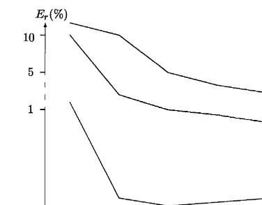
For the length of the time interval we assume T = 2 and the parameters are chosen as M = 32, M1= 100 and h∞= 0:2. Fig. 1 illustrates the relative errors Er(x; t) :=|unum(x; t)−uex(x; t)|=|uex(x; t)|
at spatial point x= (1;1:5) for the various time discretization parameter N.
For the second numerical example in the case of the direct problem the boundary 1 is given by
(4.11) and the boundary conditions are
Fig. 1. Relative errors for the various time discretization parametersN. Table 1
Numerical results for the boundary conditions (4.13) and(4.14)
x= (0;0:5) x= (1;1:5)
t M N= 10 N= 20 N= 40 N= 10 N= 20 N= 40
0.2 16 0.029736 0.024630 0.021749 0.000095 0.000063 0.000045
32 0.029736 0.024630 0.021749 0.000095 0.000060 0.000044
0.4 16 0.067445 0.064590 0.062842 0.001019 0.000903 0.000832
32 0.067445 0.064590 0.062842 0.001019 0.000898 0.000830
0.6 16 0.078015 0.078292 0.078370 0.002488 0.002386 0.002320
32 0.078015 0.078292 0.078370 0.002488 0.002384 0.002319
0.8 16 0.068023 0.069772 0.070752 0.003476 0.003441 0.003416
32 0.068023 0.069772 0.070752 0.003476 0.003442 0.003416
1.0 16 0.050837 0.052784 0.053912 0.003671 0.003692 0.003703
32 0.050837 0.052784 0.053912 0.003671 0.003694 0.003704
and
’2(x; t) =t2exp(−4(t+|x|2) + 2); (x; t)∈ 2×I: (4.14)
Table 1 gives some values for the numerical solution of the initial boundary value problem (1.1) – (1.3) at the two space points for the time interval with the length T = 1.
Now we turn to the numerical solution of the inverse problem to reconstruct the boundary 1
given by (4.11). The boundary conditions are given by (4.13) and(4.14). For the solution of the forward problem generating the ux =@u=@ on 2 we used the numerical method of Section 2.
For an approximating subspace for the radial function we choose trigonometric polynomials of degree less than or equal to K, i.e.,
q(s) =
K
X
k=0
akcosks+ 2K
X
k=K+1
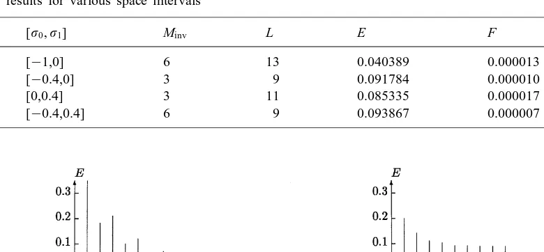
Table 2
Numerical results for various space intervals
[0; 1] Minv L E F
a [−1,0] 6 13 0.040389 0.000013 0
b [−0.4,0] 3 9 0.091784 0.000010 10−4
c [0,0.4] 3 11 0.085335 0.000017 10−5
d [−0.4,0.4] 6 9 0.093867 0.000007 10−5
Fig. 2. Relative error of the Newton iteration for casesaand b. Table 2 shows the relative error
E:=krL−r kL2[0;2]
krkL2[0;2] and the relative residual
F:=k@uL=@− kL2()
k kL2()
for various space intervals [0; 1]⊆[−1;1] and xed time interval [T0; T1] = [0;3]. The number L
counts the iteration steps required for the tolerance = 0:005.
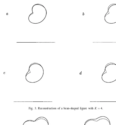
The relative errors in every Newton step for the case a andb in Table 2 are illustrated in Fig. 2. The reconstructions of the boundary 1 corresponding to Table 2 are presented in Fig. 3. The full
part of the straight line corresponds to the measurement interval [0; 1] on the innite curve 2.
For all examples the discretization parameters are M= 32, N = 20; Ninv=N and M1= 100.
The nite closed boundary 1 to be reconstructed is a peanut-shaped curve given by (3.2) with
r(s) =
q
cos2s+ 0:26 sin2(s+ 0:5); 06s62:
The boundary conditions are ’1= 0 and
’2(x; t) =t2exp(−4t+ 2); (x; t)∈ 2×I
with T = 2. Table 3 gives some numerical results for this inverse problem. The reconstructions illustrated in Fig. 4 correspond to the rst and third row of Table 3. In all our numerical experiments for the inverse problem we observe that the reconstruction is strongly dependent on the length of the space interval [0; 1] on the innite line 2 and on the distance between the reconstructed
Fig. 3. Reconstruction of a bean-shaped gure withK= 4.
Fig. 4. Reconstruction of a peanut-shaped gure withK= 4. Table 3
Numerical results for a peanut-shaped gure
[0; 1] d Minv Ninv L E F
[−2,2] 1 21 12 26 0.075709 0.000469 10−4
2 21 12 6 0.187662 0.000462 10−3
[-1;1] 1 11 20 15 0.125483 0.000393 10−4
Acknowledgements
This work was carried out whilst the author was visiting the University of Gottingen. The research was partially supported by a grant from the KAAD. The author would like to thank Professor Rainer Kress for discussions on the topic of this paper and a referee for his comments.
References
[1] H.T. Banks, F. Kojima, Boundary shape identication problems in two-dimensional domains related to thermal testing of materials, Quart. J. Appl. Math. 47 (1989) 273–293.
[2] H.T. Banks, F. Kojima, W.P. Winfree, Boundary estimation problems arising in thermal tomography, Inverse Problems 6 (1990) 897–921.
[3] Z.S. Berezhanskaya, I.V. Lyudkevich, Numerical solution of a spatial boundary value problem for the heat equation by integral equations, Vychisl. Prikl. Mat. 41 (1980) 3–7 (in Russian).
[4] C.A. Brebbia, J.C.F. Telles, L.C. Wrobel, Boundary Element Techniques, Springer, New York, 1984. [5] K. Bryan, L.F. Caudill, An inverse problem in thermal imaging, SIAM J. Appl. Math. 56 (1996) 715–735. [6] R. Chapko, R. Kress, On a quadrature method for a logarithmic integral equation of the rst kind, in: R.P. Agarwal
(Ed.), Contributions in Numerical Mathematics, World Scientic, Singapore, 1993, pp. 127–140.
[7] R. Chapko, R. Kress, Rothe’s method for heat equation and boundary integral equations, J. Integral Equations Appl. 9 (1997) 47–69.
[8] R. Chapko, R. Kress, J.-R. Yoon, On the numerical solution of an inverse boundary value problem for the heat equation, Inverse Problems 14 (1998) 853–867.
[9] D. Colton, R. Kress, Inverse Acoustic and Electromagnetic Scattering Theory, 2nd Edition, Springer, Berlin, 1998. [10] M. Costabel, Boundary integral operators for the heat equation, Integral Equations Operator Theory 13 (1990)
498–552.
[11] R. Dautray, J.-L. Lions, Mathematical Analysis and Numerical Methods for Science and Technology, Vol. 1, Physical Origins and Classical Methods, Springer, Berlin, 1990.
[12] A. Friedman, Partial Dierential Equations of Parabolic Type, Prentice-Hall, Englewood Clis, 1964.
[13] V. Galazyuk, R. Chapko, The Chebyshev-Laguerre transformation and integral equations methods for initial boundary value problems for the telegraph equation, Dokl. Akad. Nauk UkrSSR 8 (1990) 11–14 (in Russian).
[14] R.B. Guenther, J.W. Lee, Partial Dierential Equations of Mathematical Physics and Integral Equations, Prentice-Hall, Englewood Clis, 1988.
[15] G.C. Hsiao, J. Saranen, Boundary integral solution of the two-dimensional heat equation, Math. Meth. Appl. Sci. 16 (1993) 87–114.
[16] R. Kress, Linear Integral Equations, Springer, Berlin, 1989.
[17] R. Kress, I.H. Sloan, On the numerical solution of a logarithmic integral equation of the rst kind for the Helmholtz equation, Numer. Math. 66 (1993) 199–214.
[18] O.A. Ladyzenskaja, V.A. Solonnikov, N.N. Uralceva, Linear and Quasilinear Equations of Parabolic Type, AMS Publications, Providence, 1968.
[19] N.N. Lebedev, Special Functions and Their Applications, Prentice-Hall, Englewood Clis, 1965.
[20] C. Lubich, R. Schneider, Time discretizations of parabolic boundary integral equations, Numer. Math. 63 (1992) 455–481.