SPECIAL ISSUE
THE VALUES OF WETLANDS: LANDSCAPE AND INSTITUTIONAL
PERSPECTIVES
Economic criteria for using wetlands as nitrogen sinks under
uncertainty
Olof Bystro¨m
a,*, Hans Andersson
a, Ing-Marie Gren
a,b aDepartment of Economics,Swedish Uni6ersity of Agricultural Sciences,Box7013,S75007Uppsala,Sweden bBeijer International Institute of Ecological Economics,The Royal Swedish Academy of Sciences,Box50005,S10405Stockholm,Sweden
Abstract
If the environmental damages that are caused by excessive nitrogen load to the sea depend on the timing of emissions, then monitoring the stochastic variation of emissions is crucial for controlling eutrophication damages. A significant problem of nonpoint source (NPS) nitrogen pollution is that emissions are stochastic and difficult to control. The main purpose of this paper is to examine under what criteria wetlands are economically rational to use for controlling stochastic NPS pollution. Three criteria are identified using a simplified stochastic watershed model. It is suggested that wetlands are economically rational to use, especially when monitoring the uncertainty of emissions is a part of the decision problem. The theoretical findings are illustrated with an example from southwestern Sweden. © 2000 Elsevier Science B.V. All rights reserved.
Keywords:Chance constraints (CCP); Costs; Nitrogen abatement; Swedish wetlands; Stochastic; Uncertainty
www.elsevier.com/locate/ecolecon
1. Introduction
Over the past decade, the use of wetlands for abatement of point and nonpoint source pollution has received substantial attention in the literature (e.g. Folke, 1990; Hammer, 1992; Gren, 1993; Mitsch and Gosselink, 1993; Jansson et al. 1994). From an economic perspective, wetlands have been suggested as a low cost measure to reduce
point and nonpoint pollution (Folke, 1990; Gren, 1993; D’Angelo and Reddy, 1994; Gren, 1995). However, none of the previous studies have ad-dressed the issue of uncertainty in relation to the economics of wetland restoration. If environmen-tal damages are created partly by peak loads of pollutants, such as seasonal and annual variations in nitrogen load to the sea, then it is of vital importance to monitor the uncertainty of emis-sions. Consequently, addressing the uncertainty of wetlands’ abatement capacity and impact on the overall uncertainty of nonpoint pollution may * Corresponding author. Fax: +46-18-673502.
E-mail address:[email protected] (O. Bystro¨m).
have implications for the economic relevance of wetlands, and for implementing economic policies designed to control point and nonpoint source pollution.
In this paper we examine under what conditions wetlands are economically rational to use for abatement of nonpoint nitrogen pollution, recog-nizing that agricultural run-off as well as the nitrogen abatement capacity of wetlands are stochastic. Economic criteria for wetlands are es-tablished using a simplified theoretical model of a watershed. In contrast to previous studies on wet-lands, we extend the analysis by explicitly model-ing the uncertainty of nonpoint emissions and the uncertainty of nitrogen abatement in wetlands. The implications of uncertainty on the conditions for optimal nitrogen abatement in a watershed are discussed, and an example from southwestern Sweden is used to illustrate and evaluate the theoretical findings.
2. The model
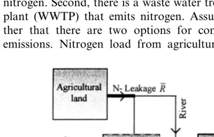
To establish economic criteria for construction of wetlands under uncertainty, consider a water-shed in which there are two sources of nitrogen emissions. First, there are agricultural emissions resulting in nonpoint source (NPS) emissions of nitrogen. Second, there is a waste water treatment plant (WWTP) that emits nitrogen. Assume fur-ther that fur-there are two options for controlling emissions. Nitrogen load from agricultural land
may be reduced by construction of wetlands that are designed for nitrogen abatement. Point source emissions from the WWTP may be reduced by investments in waste water treatment. This sim-plified watershed is illustrated in Fig. 1 below. While it is recognized that NPS emissions are stochastic, the model is simplified by assuming that emissions from the WWTP are deterministic. This assumption accommodates the plausible fact that emissions from nonpoint sources are charac-terized by a high variability, compared to emis-sions of the WWTP, due to climate, precipitation, and other factors (Malik et al., 1993).
The level of nitrogen leakage from agricultural land depends on management practices and on stochastic events such as temperature and precipi-tation (Shortle and Dunn, 1986). Leakage is thus stochastic and in this paper denoted byR0. Part of the agricultural leakage enters wetlands, thus making nitrogen abatement in wetlands stochas-tic. In addition, the abatement capacity of a wet-land depends on weather and is consequently stochastic in itself (Mitsch and Gosselink, 1993). Finally, since both abatement in wetlands and leakage from agricultural land are stochastic, the total nitrogen load from the watershed to the sea is a stochastic variable.
To model nitrogen retention in wetlands, a denitrification model developed in Bystro¨m (1998), is utilized.1 Denoting retention (abate-ment) in wetlands byQ0 and total nitrogen load by P0, both of which are stochastic, the following definitions are established:
R0 =(r+o0)(L( −Lw) (1)
Q0 =(a+o1)Lw+bR0s (2)
P0 =R0 −Q0 +Z (3)
where,
Fig. 1. Watershed model displaying the structure of the prob-lem and the variables used.
r=Expected nitrogen L( =Maximum area of
agricultural land. leakage per hectare of agricultural land.
It is assumed in this paper that the random errors, o0 and o1, are independent and normally distributed. By the notation chosen in Eq. (1) it is clear that we assume that there can be no idle land in the watershed, all agricultural land is used either as wetlands or for cultivation of crops.2
The watershed is modeled from the perspective of a regulatory agency, where the objective is to maximize economic return from the watershed area, subject to a pollution constraint. If environ-mental damages of excessive nitrogen emissions are caused not only by a high level of expected nitrogen load, but also by random peak flows, then monitoring the uncertainty of emissions be-comes important for controlling environmental damages. Consequently, the distribution of emis-sions needs to be reflected in the pollution con-straint. One approach to incorporate uncertainty into standard models of constrained optimization is to require that the environmental pollution constraint is achieved by a certain probability. By specifying an acceptable probability level, it is possible to monitor the risk of violating the pollu-tion constraint. Recognizing that the abatement target has to be achieved with a certain probabil-ity, the decision problem can be modeled as follows:
p=Per hectare profit P*=Pollution of crop cultivation on constraint. agricultural land.
C(Lw)=Cost function a=Probability by for construction of which the pollution
constraint should be
The probabilityaspecifies the minimum proba-bility according to which the pollution constraint,
P*, should be satisfied. If a equals 0.5, then
pollution constraint (5) is equivalent to incorpo-rating the deterministic constraint of reducing solely expected emissions. If, however, a is be-tween 0.5 and 1, constraint (5) requires that the abatement target is achieved by a probability level exceeding that of reducing only expected emis-sions. Thus, constraint (5) effectively specifies a reliability constraint that the policy planner may address by imposing additional restrictions on expected emissions or by improving the distribu-tion of total emissions.
A convenient approach for solving the decision problem specified by (4) and (5) is to use the chance constrained programming approach which has been commonly applied for solving economic programming problems under uncertainty (e.g. Charnes and Cooper, 1964; McSweeny and Shortle, 1990; Shortle, 1990). The problem formu-lation under this approach is useful for illustrating the impact of uncertainty, and how the variance of emissions affects the optimal solution. The method makes it possible to replace the proba-bilistic pollution constraint with its deterministic equivalent, such that standard deterministic opti-mization methods can be applied. Following Mc-Sweeny and Shortle (1990) and Paris and Easter 2Furthermore, with the chosen modeling approach, the
Table 1
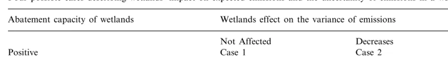
Four possible cases describing wetlands’ impact on expected emissions and the uncertainty of emissions in a watershed Abatement capacity of wetlands Wetlands effect on the variance of emissions
Not Affected Decreases Increases
Case 3 Case 2
Positive Case 1
None/negative Case 4 Case 4 Case 4
(1985), the constraint in Eq. (5) is rewritten as a chance constraint3:
E(P)+faV(P)
1/25P* (6)
where E(P) is the expected nitrogen load,V(P)=
V(R)+V(Q)−2Co6(Q,R) is the variance of total
nitrogen load andfais a parameter that specifies the weight that should be attached to the variance of emissions in order for the abatement target to be reached with a probability a (Taha, 1976). In this paper it is assumed that V(P) follows a normal distribution. For a given probability, the value of fa is then obtained from the standard normal cumulative distribution. If uncertainty of emissions is irrelevant to the problem, then fa is equal to zero (i.e.a=0.5). If, however, the uncer-tainty is to be monitored, that isa\0.5, then fa is positive, thus including the variance into the pollution constraint. Consequently, pollution con-straint (6) becomes stricter with increasing reli-ability requirements. It is obvious from Eq. (6) that there are two main strategies for reducing the nitrogen load such that the abatement target is not violated. First, the strategy may address abatement efforts that are mainly directed to-wards reducing the average, or expected, emis-sions, E(P). Secondly, abatement measures that are mainly designed to reduce uncertainty, and thus the variance, of emissions may be used. Since WWTP emissions are assumed to be deterministic, a reduction of these emissions affects only the expected nitrogen load. In this paper wetlands represents a strategy that affects the uncertainty
of nitrogen load to the sea. As a consequence, criteria for the economic relevance of wetlands include not only the expected abatement and the construction costs thereof, as have been shown in previous studies (e.g. Bystro¨m, 1998; Gren, 1993, 1995), but more so the impact of wetlands on the uncertainty of nitrogen load to the recipient.
Unless anything specific is known about wet-lands’ abatement capacity, or impact on the vari-ability of nitrogen load, there are four possible cases that may characterize wetlands’ impact on water quality in the watershed. These scenarios are displayed in Table 1.
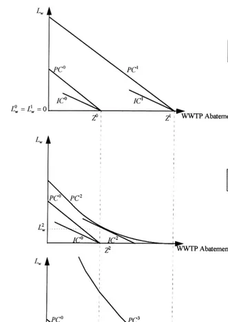
Clearly, in the event that case 4 prevails, wet-lands are never economically rational in terms of nitrogen abatement, irrespective of costs. How-ever, do any of the other situations rule out wetlands as an economically relevant abatement measure? To address this question, let us examine the optimal solution to the pollution problem graphically for the three first situations. Fig. 2a – c display the optimal solutions and the constraints to the models. Each scenario is referred to by its number.
In Fig. 2a, IC0is an isocost curve that describes all combinations of wetlands and WWTP abate-ment that yield a constant total cost. If both construction costs for wetlands and the costs of WWTP reductions are linear, then IC0 is linear. IC1
– IC3
are defined analogously although they depict different total costs. Costs increase as the IC curve shifts out from the origin, since costs increase in construction of wetlands, and with increased reduction of WWTP emissions. The slope of the IC-curves is equal to the relative marginal cost between emission reductions in WWTPs and construction of wetlands. PC0
– PC3 denote pollution constraints. The PC-curves define all combinations of wetlands and WWTP 3For a description of the general approach and the
Fig. 2. Optimal allocation of abatement under three scenarios. abatement that correspond to a specific
pollu-tion constraint. PC0 denotes the pollution con-straint when uncertainty of emissions is not considered (a=0.5, f
a=0). The optimal alloca-tion of abatement efforts can be observed in the figures as the point where an IC-curve is
tan-gent to the pollution constraint, or where the intersection between the curves yields the lowest total costs. For the base case when only ex-pected nitrogen loads are considered (fa=0), the optimal solution is given by (Z0
, Lw0
When the pollution constraint is to be satisfied with a probability greater than 0.5, the PC-curve shifts out, since including the variance now re-quires increasing abatement efforts. Fig. 2a de-picts case 1, when construction of wetlands does not affect the uncertainty of emissions. In this case there are no possibilities to affect the vari-ance of emissions, and thus the only possibility is to reduce expected emissions such that the modified pollution constraint, PC1, is not vio-lated. It can be noted that the curvature and the slope of pollution constraint PC1
is identical to the original PC0
, since neither WWTP reductions nor construction of wetlands affect the distribu-tion of nitrogen load. The optimal allocadistribu-tion in case 1 is given by (Z1,
Lw
1).
Fig. 2b depicts case 2. Under this scenario construction of wetlands reduces the variability of total nitrogen load. This means that wetlands become more efficient with respect to fulfilling the abatement target, compared to case 1 (see also Eq. (6)). If the variance-reducing effect of wet-lands is higher for the first units of wetwet-lands constructed, then the pollution constraint PC2 is convex as shown in the figure (this is formally shown in the appendix to this paper). Hence, a higher emission reduction is required in the waste water treatment plant in order to substitute for one unit of nitrogen reduction in wetlands com-pared to case 1. The optimal combination of wetlands and WWTP reductions is now given by (Lw
2, Z2). The total cost is in this case given by
IC2, which is lower than the total costs in the first case of Fig. 2a.
The scenario under case 3 is shown in Fig. 2c. In this case construction of wetlands increases the uncertainty of emissions. If the rate of augmenta-tion in variance increases as larger areas of wet-lands are constructed, then the pollution constraint in case 3 is convex as indicated in Fig. 2c (this is shown in the appendix). The effect on the pollution constraint as defined by Eq. (6) is in this case ambiguous and it is unclear whether construction of wetlands contributes to solving the pollution problem. In this scenario wetlands are less efficient compared to the situation when construction of wetlands does not affect the vari-ance, fewer units of WWTP reductions are
re-quired to substitute for one unit of nitrogen reduction in wetlands.
The three cases above depict the possible cases for wetlands in theory. In practice it can be expected that one of these situations prevails. But in which of the cases are wetlands economically relevant to use for nitrogen abatement, and in which case is the relevance of wetlands unambigu-ous? Under case 4, wetlands are clearly not eco-nomically relevant, since wetlands neither perform abatement, nor improve the distribution of emis-sions. Therefore case 4 can be ruled out directly. In case 3 wetlands have a positive abatement capacity, but construction of wetlands also in-creases the variability of total emissions, which makes the overall abatement effect uncertain, at least when the abatement target is to be achieved with some degree of certainty (a\0.5,fa\0). In case 1 and 2 the expected abatement capacity of wetlands is positive. Moreover, in case 2 the abatement capacity, or the economic relevance, of wetlands increases with the introduction of a reli-ability requirement since wetlands in case 2 also reduce the uncertainty of emissions. In this case the abatement performed by wetlands is unam-biguous, and the abatement capacity is not dimin-ished if stricter reliability constraints are imposed. Three criteria for the economic relevance of using wetlands for nitrogen abatement can now be formulated.
The abatement capacity of wetlands must be
positive and increasing in wetland area.
The use of wetlands for nitrogen abatement
must not increase the uncertainty, or variance, of total nitrogen load.
Given that the two first conditions are fulfilled,
we also require that wetlands have sufficiently low abatement costs to be considered as a viable measure for pollution reduction in nitro-gen abatement programs. The relative prices are given by the slope of the IC-curves in Fig. 2a – c.
3. Economic policy and wetlands
the analysis of abatement costs means that wet-lands’ effect on the total variability of emissions influences the optimal allocation of abatement between point and nonpoint emissions. This is clearly displayed in Fig. 2 where the optimal area of wetlands varies, depending on the prevailing situation. Knowledge of how the use of wetlands affects uncertainty may therefore be crucial for identifying to what extent wetlands are beneficial to use for nitrogen abatement. Moreover, if the criteria of economic relevance are fulfilled, it can be shown that a stricter reliability require-ment implies that the pollution constraint shown in Fig. 2b becomes more convex (McSweeny and Shortle, 1990). Consequently, an extended use of wetlands is suggested the stricter the reliability constraint. This result is a consequence of wet-lands, in this paper, being the only means by which the uncertainty of total emissions can be reduced.
The second implication of the criteria above is perhaps more subtle. If the criteria are fulfilled, the use of wetlands reduces the uncertainty of nonpoint emissions. In addition, parts of the upstream nonpoint emissions are gathered in wetlands and the net emissions can be measured at the downstream exit of a wetland. Thus, construction of wetlands may in fact contribute to changing some of the characteristics of the nonpoint emissions in the watershed. Nonpoint emissions are characterized by their uncertainty and the difficulty by which they can be measured and monitored (Malik et al. 1993; Shortle and Dunn, 1986). Wetlands reduce uncertainty and provide a natural point at which the upstream pollution can be measured. In this respect we can therefore conclude that wetlands are ‘pointifiers’ of nonpoint emissions, i.e. an abate-ment measure that makes nonpoint emissions assume the characteristics of point source emis-sions. Since some of the upstream pollution can be measured as the outflow from the downstream exit of a wetland, construction of wetlands implies that a portion of the upstream nonpoint emissions can be measured and monitored as point sources.
4. Example
To illustrate the implications of the criteria established above, this section provides an exam-ple of a stylized watershed using empirical data from southwestern Sweden. This is a region with relatively high leakage of nitrogen due to intensive agriculture and sandy soils (Johnsson and Hoff-mann, 1997). Although the watershed is rather simplified, we use empirical data concerning costs, agricultural yields, and nitrogen leakage. The out-line of this model follows the schematic illustra-tion in Fig. 1. It is assumed that there is one representative farm in a watershed that emits nitrogen through agricultural run-off or leakage, and that wetlands is the only measure by which the nitrogen load to the sea from leakage can be reduced. Finally, there is one WWTP that emits nitrogen directly into the coastal zone. The objec-tive of the policy maker is to maximize economic return in the area, subject to a probabilistic pollu-tion constraint. The abatement target that is used in this paper is a 30% reduction of the nitrogen load to the sea. The problem is formulated as maximizing (4), subject to (6), and additional constraints regulating the maximum area of wet-lands and the minimum level of WWTP emissions.
4.1. Data and assumptions
Table 2
Characteristics of the hypothetical watersheda
Wetlands
Agricultural land Waste water treatment plant
6600 –
Initial emissions (kg year−1) 7000
– 10
Maximum area (ha) 200
0 0.76
Variance coefficient 0.35
– –
Variable profit (SEKbha−1year−1) 2242
– 12518 ha−1 44 kgN−1 Costs (SEKbyear−1)
Initial marg. abatem cost (SEK kgN−1 year−1) – 54 44
aSources: Bystro¨m (1998), Gren et al. (1997), Vatn et al. (1996), Johnsson and Hoffmann (1997), and SLU (1995). bSEK, 0.12 USD ( January 2000).
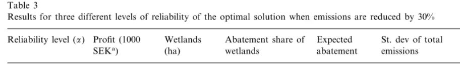
Table 3
Results for three different levels of reliability of the optimal solution when emissions are reduced by 30%
Reliability level (a) Profit (1000 Wetlands Abatement share of Expected St. dev of total Variance coefficient emissions
(ha) abatement
SEKa) wetlands
50% 269 0.0 0% 30% 2470 0.26
75% 193 1.2 5% 42% 2320 0.29
0.22
144 30% 46% 1660
90% 8.1
aSEK, 0.12 USD ( January 2000).
Data to characterize the watershed are obtained from various sources. The costs for construction of wetlands, together with the abatement capacity and the uncertainty of nitrogen abatement in wet-lands, are obtained from Bystro¨m (1998).4 Data for yield and profitability of crop cultivation are obtained from SLU (1995), and the costs of in-creased nitrogen abatement in WWTPs are ob-tained from Gren et al. (1997). Finally, data concerning leakage of nitrogen from agricultural land are obtained from Johnsson and Hoffmann (1997). Estimates of the variability of leakage from cultivation of wheat are not available for Swedish soils. Therefore data from a Norwegian study is used and it is assumed that the variance coefficient for nitrogen leakage is the same in
Sweden as for the soils in the Norwegian study (Vatn et al., 1996). Using these data and assump-tions, the background information used to model the watershed is summarized in Table 2.5
4.2. Results
To show how reliability constraints influence the pollution constraints, and the array of feasible solutions, the model is solved for three different levels of reliability. First the model is solved de-terministically, such that the variance of total emissions does not influence the solution (a=
0.5). Second, the model is solved for two levels of reliability such that the variance receives different weight in the pollution constraint (a=0.75, and a=0.9). As mentioned above, the required level
of reliability affects the restrictiveness and the convexity of the pollution constraint as defined by Eq. (6). The results for each of the reliability levels imposed are displayed in Table 3.
The optimal allocation between abatement in wetlands and emission reductions in the WWTP varies depending on the level of reliability spe-cified. Table 3 shows that the level of required 4It is perhaps noteworthy that in this paper we use
Bystro¨m’s linear model of denitrification (see Eq. (2)), since it is easier to calculate the uncertainty and the covariance be-tween agricultural land and wetlands if a linear model is used. The parameter values of Eq. (2) used for this example are a=167.5, andb=0.079 (Bystro¨m, 1998).
certainty has a substantial impact on the optimal solution. As a increases, monitoring the uncer-tainty of emissions becomes increasingly impor-tant. Therefore the optimal use of wetlands increases with increased reliability requirements. The abatement efforts are now ‘switched’ from point to nonpoint abatement due to the capacity wetlands have to reduce the uncertainty of non-point emissions. Table 3 also shows that imposing reliability requirements is costly. Profits are re-duced by approximately 50% when a reliability level of 90% is required, compared to the case when only the expected nitrogen load is relevant to the problem.
The example is based on empirical values that are more or less uncertain. To analyze the sensi-tivity of the solution to changes, the parameter values that are relevant to the economic criteria established were changed. Table 4 displays the optimal area of wetlands when the cost, abate-ment capacity, and variance parameters are changed.
It is clear from Table 4 that the optimal solu-tion is sensitive to changes in all the parameters evaluated, regardless of reliability level. A de-crease in costs or an inde-crease in wetlands’ abate-ment capacity increases the optimal area of wetlands quite substantially. The correlation co-efficient between the nitrogen abatement in wet-lands and runoff from agricultural land affects the covariance between wetlands and agricultural land (COV(Q,R)). In this paper it is assumed that the correlation is 0.7. Reducing this parameter to
0.5 (−25%) makes wetlands less attractive to use in the solution. Due to the sensitivity to changes in the parameters, it is difficult to draw any decisive conclusions from the empirical model regarding the economic relevance of wetlands un-der uncertainty. However, all of the parameter changes that are displayed in Table 4 are con-nected to the economic criteria established in the theoretical section of this paper. Therefore the empirical results suggest that the established crite-ria captures the main determinants of whether wetlands are economically rational to use for nitrogen abatement. Consequently, the established criteria are of importance for determining whether or not wetlands should be restored in a particular region.
5. Conclusions
This paper aims to identify under what condi-tions wetlands are economically relevant to use for abatement of nonpoint nitrogen emissions. Criteria are established for the economic rele-vance of wetlands, recognizing that nonpoint emissions as well as their abatement are stochas-tic. Uncertainty is explicitly accounted for and it is shown that the level of uncertainty may be of decisive importance for the economic relevance of wetlands.
Three criteria are established: first, the use of wetlands for nitrogen abatement must not in-crease the variability of total nitrogen emissions; second, the abatement capacity of wetlands must be positive and increasing in wetland area; and finally, given that the first two criteria are fulfilled, the abatement costs must be sufficiently low to motivate construction of wetlands as a part of a cost-effective nitrogen reduction program. It can be verified in the literature that these conditions are generally fulfilled.6
The empirical part of this Table 4
Sensitivity analysis
Optimal area of wetlands (ha)
a=75% a=90%
a=50%
8.1
Base case 0.0 1.2
4.2
Wetland costs−25% 10 10
Correlation coeff.−25% 0.0 0.0 4.7 8.9 0.0
0.0 St. dev. of stochastic
variables:−25%
0.0
Abatement capacity+25% 9.7 10.0
paper uses data from southwestern Sweden. It is shown that the optimal use of wetlands is sensitive to changes in both the underlying assumptions and the empirical values used to model the water-shed. Although conclusive empirical evidence for the economic relevance of wetlands is difficult to establish on the basis of data used in this article, the established criteria specify the main sources of sensitivity. Consequently, the established criteria are important for identifying economically viable wetlands for nitrogen abatement.
Appendix A
Given the definitions of nitrogen leakage and retention in wetlands, we can define the variance of total emissions, denotedV(P), according to the following:
are the variances of the stochas-tic variables defined in Eq. (1) and Eq. (2), and s0,1 describes the covariance between agricultural land and wetlands. To clarify wetlands’ effect on the variance, Eq. (7) is differentiated with respect to wetland area.
Clearly Eq. (8) can be both positive and nega-tive depending on which of the variances domi-nate the derivative. Finally, to determine whether the pollution constraints in Fig. 2 are concave or convex, the second derivative of Eq. (7) with respect to wetland area is determined:
(V2(P)
(L w
2 =2s02(1−bs)2+2s12+4s0,1(1−bs) (9)
It is clear Eq. (9) is a positive constant. Since E(P) is linear, Eq. (9) demonstrates that the pol-lution constraint defined by Eq. (6) is convex, irrespective of whether construction of wetlands increases or decreases the variance of total
emis-sions. This result follows from the quadratic defi-nition of a variance (Greene, 1993).
References
Arheimer, B., Wittgren, H.B., 1994. Modeling the effects of wetlands on regional nitrogen transport. Ambio 23, 378 – 386.
Bystro¨m, O., 1998. The nitrogen abatement cost in wetlands. Ecolog. Econ. 26, 321 – 331.
Charnes, A., Cooper, W.W., 1964. Deterministic equivalents for optimizing and satisfying under chance constraints. Oper. Res. 11, 18 – 39.
D’Angelo, E.M., Reddy, K.R., 1994. Diagenesis of organic matter in a wetland receiving hypereutrophic lake water. II. Role of inorganic electron acceptors in nutrient release. J. Environ. Qual. 23, 937 – 943.
Folke, C., 1990. Evaluation of ecosystem life-support in rela-tion to salmon and wetland exploitarela-tion, Deptartment of Systems Ecology. University of Stockholm, Stockholm. Greene, W.H., 1993. Econometric Analysis, second ed.
MacMillan Publishing Company, New York.
Gren, I.M., 1993. Alternative nitrogen reduction policies in the Ma¨lar region, Sweden. Ecol. Econ. 7, 159 – 172.
Gren, I.M., 1995. The value of investing in wetlands for nitrogen abatement. Euro. Rev. Agric. Econ. 22, 157 – 172. Gren, I.M., Elofsson, K., Jannke, P., 1997. Cost-effective nutrient reductions to the Baltic Sea. Environ. Res. Econ. 10, 341 – 362.
Hammer, D.A., 1992. Designing constructed wetlands systems to treat agricultural nonpoint source pollution. Ecol. Eng. 1, 49 – 82.
Jansson, M., Andersson, R., Berggren, H., Leonardsson, L., 1994. Wetlands and Lakes as Nitrogen Traps. Ambio 23, 320 – 325.
Johnsson, H., Hoffmann, M., 1997. Nitrogen Leakage from Swedish Agricultural Land. Swedish Environmental Pro-tection Agency, Stockholm.
Leonardsson, L., 1994. Va˚tmarker som kva¨vefa¨llor, Svenska och internationella erfarenheter. Swedish Environmental Protection Agency, Solna.
Malik, A.S., Letson, D., Crutchfield, S.R., 1993. Point/non-point source trading of pollution abatement: choosing the right trading ratio. Am. J. Agric. Econ. 75, 959 – 967. McSweeny, W.T., Shortle, J.S., 1990. Probabilistic cost
effec-tiveness in agricultural nonpoint pollution control. S. J. Agric. Econ. 22, 95 – 104.
Mitsch, W., Gosselink, J.G., 1993. Wetlands, second ed. Van Nostrand Reinhold, New York.
Paris, Q., Easter, C.D., 1985. A programming model with stochastic technology and prices: the case of Australian agriculture. Am. J. Agric. Econ. 67, 120 – 129.
Shortle, J.S., Dunn, J.W., 1986. The relative efficiency of agricultural source water pollution control policies. Am. J. Agric. Econ. 68, 668 – 677.
SLU, 1995. Omra˚deskalkyler-Jordbruk GSS 1995/96. Swedish University of Agricultural Sciences, Uppsala.
Taha, H.A., 1976. Operations Research, and introduction, second edn. Macmillan Publishing, Inc, New York. Vatn, A., Bakken, L.R., Bleken, M.A., et al., 1996. Policies for
reduced Nutrient Losses and Erosion from Norwegian Agriculture. A,s Science Park Ltd, Norway.