Manajemen | Fakultas Ekonomi Universitas Maritim Raja Ali Haji 073500103288618936

Full Terms & Conditions of access and use can be found at

http://www.tandfonline.com/action/journalInformation?journalCode=ubes20

Download by: [Universitas Maritim Raja Ali Haji] Date: 13 January 2016, At: 00:47

Journal of Business & Economic Statistics

ISSN: 0735-0015 (Print) 1537-2707 (Online) Journal homepage: http://www.tandfonline.com/loi/ubes20

Efficient Estimation of Semiparametric

Equivalence Scales With Evidence From South

Africa

Adonis Yatchew, Yiguo Sun & Catherine Deri

To cite this article: Adonis Yatchew, Yiguo Sun & Catherine Deri (2003) Efficient Estimation of

Semiparametric Equivalence Scales With Evidence From South Africa, Journal of Business & Economic Statistics, 21:2, 247-257, DOI: 10.1198/073500103288618936

To link to this article: http://dx.doi.org/10.1198/073500103288618936

View supplementary material

Published online: 24 Jan 2012.

Submit your article to this journal

Article views: 63

View related articles

Ef’cient Estimation of Semiparametric

Equivalence Scales With Evidence

From South Africa

Adonis

Yatchew

_{, Yiguo}

Sun

_{, and Catherine}

Deri

University of Toronto, Toronto, Canada M5S 3G7

(yatchew@chass.utoronto.ca) (yiguosun@chass.utoronto.ca) (cderi@chass.utoronto.ca)

We propose semiparametric procedures for estimation and testing of base-independent equivalence scales. The partial linear index speciŽcation permits simultaneous estimation across multiple household types and multiple goods and also the incorporation of continuous and discrete household attributes. Furthermore, asymptotic properties of estimated equivalence scales and tests of base independence are readily obtained. The efŽciency gains from the proposed models and estimators are particularly helpful for developing country data where there is often much greater variation in household size and composition. We apply the techniques to South African data and Žnd the results to be broadly consistent with base independence.

KEY WORDS: Base independence; Equivalence scales; Partial linear index model.

1. INTRODUCTION

In recent papers, Blundell, Duncan, and Pendakur (1998) and Pendakur (1999) proposed semiparametric estimators of base-independent equivalence scales. Suppose that there are two types of households, A and B. Letxbe household expen-diture and letpbe a vector of prices corresponding to goods purchased. For the moment we will focus on purchases of a single good, say food. Let y_A Df_A4p1 x_A5 be the food share of expenditure for households of type A. Under base-independence, the food share of type B households is related to that of type A households by

yBDfB4p1 xB5DfA ³

p1 xB

ã_B4p5

´

CÇB4p5 (1)

where ã_B4p5 is the base-independent equivalence scale and

Ç_B is its elasticity with respect to the price of food. (See Pendakur 1999, p. 5, eq. 2.5, which draws on earlier work in Lewbel 1989 and Blackorby and Donaldson 1989, 1993, 1994.) Such scales—if valid—are extremely convenient, because they tell us how much income is required by holds of type B to achieve the same level of utility as house-holds of type A, that is,xBDãB4p5¢xA. Holding prices

con-stant, expenditure shares as a function of the log of income are vertical and horizontal translations of each other,

yBDfB4xB5DfA ³

xB

ã_B

´

CÇBDf 4logxBƒÄB5CÇB1 (2)

where Ä_B Dlogã_B and f Df_Ažexp, a convolution of the type A share function with the exponential function. Pendakur tested this translation “shape invariance” while estimating the function f nonparametrically. To do so, he drew on ear-lier results of H¨ardle and Marron (1990, 1993), Pinkse and Robinson (1995), and others. His analyses were restricted to pairwise comparisons of household types. Because validity of equivalence scales requires that they be the same for each expenditure category, he also performed analyses across mul-tiple goods. This has the added beneŽt of improving efŽciency of estimation of the equivalence scale parameterÄB.

The estimation of share functions and shift parameters may be equivalently cast into a partial linear index function frame-work, (see in particular Carroll, Fan, Gijbels, and Wand 1997, as well as Ichimura 1993; Powell 1994; Horowitz and H¨ardle 1996; Cavanagh and Sherman 1998; and references therein). Suppose that there areqC1 family types, and select the Žrst type as the reference to which the otherq types will be com-pared. Let z be aq-dimensional row vector of dummy vari-ables for the q (nonreference) family types, and let Øbe an iid random variable with mean 0 and varianceÑ2_{. Then under} the null hypothesis that there exists a base-independent equiv-alence scale, we may write:

yDf 4logxƒzÄ5CzÇCØ1 (3)

whereÄandÇareq-dimensional parameter vectors. Blundell et al. (1998) proposed such a framework, which they call the extended partial linear model, but perform estimation and test-ing ustest-ing only pairs of household types. Their procedures and those of Pendakur (1999) and Gozalo (1997) are valid in het-eroscedastic settings. For purposes of identiŽcation, the coefŽ-cient of logxis set to 1. Within this framework, it is straight-forward to conduct analyses across multiple household types (and multiple goods). For example, one can test whether all qC1 family types can be embedded in a common model of the form (3), whether families with and without children require separate speciŽcations, or whether all family types are funda-mentally different. Whereas Pendakur (1999) relied on sim-ulation methods to obtain standard errors and critical values, the partial linear index model framework—while not preclud-ing simulation—permits one to adapt existpreclud-ing estimation and testing results to produce asymptotically valid procedures.

To estimate the equivalence scale and elasticity as well as the nonparametric function f, we adapt a symmetric

©2003 American Statistical Association Journal of Business & Economic Statistics April 2003, Vol. 21, No. 2 DOI 10.1198/073500103288618936 247

k–nearest-neighbor smoother to the partial linear index model setting. The procedure is simple to implement and computa-tionally fast as long as the number of distinct family types is small. However, the computational burden does increase withq. The reason is that estimation of index model param-eters (in our case, Ä) typically requires a grid search. (See Horowitz and H¨ardle 1996 for an alternative procedure.)

In Canada, about 75% of the population lives in households that consist of singles or couples with 0, 1, or 2 children (a total of 6 family types). In contrast, in developing countries one tends to observe much larger variation in household size and composition. Couples tend to have more children, and it is not uncommon for extended families to occupy a single household. For example, for South Africa, which we study in some detail herein, less than 40% of the population lives in the types of families just listed. Restricting attention to these six family types would ignore most of the population. To build a parsimonious model that can handle a large number of family types while maintaining semiparametric exibility, consider the following speciŽcation for the equivalence scale:

ãD4ACÂ₂K5Â1_{1 (4)}

whereAis the number of adults in the household andKis the number of children. Here Â₁ reects scale economies in the household andÂ₂measures the effect on the equivalence scale of children relative to adults. Both parameters are restricted to be between 0 and 1. (See, e.g., Citro and Michael 1995, p. 176, who recommended values around .7 for Â1 and Â2.) Using (4), our model becomes

yDf 4logxƒÂ1log4ACÂ2K55CzÇCØ0 (5)

Although estimation of (3) requires a q-dimensional grid search to estimate Ä, (5) reduces this search to two dimen-sions. (No similar problem exists for estimation of Ç.) Fur-thermore, because the equivalence scales are functions of only two parameters, they will generally be estimated more pre-cisely. Finally, speciŽcation (5) has the appealing property that it is monotone inA andK and yields plausible “spacings” of equivalence scales among families of similar composition. Of course, from an equity standpoint, what is required is accu-racy. We test the speciŽcation later in the article.

In our parsimonious model, we propose a particularly sim-ple speciŽcation for the equivalence scale, (4). Variables A andK are both discrete, but more complicated speciŽcations incorporating both discrete and continuous variables (such as age) can be estimated using the procedures outlined herein. After delineating estimators for models (3) and (5), we pro-duce a simple test of base independence (which is essentially a test of whether the share functions coincide after horizon-tal and vertical translation) and a test of the parsimonious speciŽcation (5) against the more general (3). The tests com-pare restricted and unrestricted residual variance estimates. If reliable data are available on the consumption of various goods, then system estimation may be applied, because the equivalence scale parameter is common across share equations for different goods. This can be implemented most easily by applying generalized least squares (GLS) methods to the sin-gle equation estimates, but we also use systemwide estimation

procedures. A simple chi-squared test may then be applied to test the equality of equivalence scale parameters across goods. The article is organized as follows. Single-equation and multiequation estimators and test procedures are described in Section 2. These techniques are applied to South African data on food and rent expenditures in Section 3. The estimates obtained in Section 3 are then used to perform efŽciency com-parisons of various speciŽcations in Section 4. Our principal focus is on the equivalence scale parameterÄ, because this is usually of greatest interest. We Žnd up to a 25% improvement in efŽciency when estimating the multifamily model (3) rela-tive to pairwise estimation. In comparison, the parsimonious model (5) yields as much as a fourfold increase in precision. Multiequation estimation (using food and rent data) yields modest gains of less than 5%. An Appendix contains technical results. (For additional details and Monte Carlo experiments see Yatchew, Sun, and Deri 2000.)

2. STATISTICAL PROCEDURES

2.1 Single-Equation Estimation

Suppose that we are given data4y11 x11 z151 : : : 1 4yn1 xn1 zn5

on nhouseholds. With mild abuse of notation, we use y and x to denote both the variable in question and the correspond-ing column vector of observations on the variable. The con-text should make it clear which one applies. Ifx is a vector, then f 4x5denotes the vector consisting off evaluated at the components ofx0 We useZto denote thenxqmatrix of data on the dummy variables. Hence logxƒZÄis a vector, as is f 4logxƒZÄ5. Equation (3) may be written in vector-matrix notation as

To estimate this model, we rely on the symmetric k– nearest-neighbor smoother (also known as the running mean smoother), which averages an equal number of observations on either side of a point to estimate the function at that point. (Assume throughout thatk is even.) The estimator is fast and simple to implement. Thus, let S be the smoothing matrix given by

Analogously to work of H¨ardle, Hall, and Ichimura (1993), the same asymptotically optimal smoothing parameterk may be used to estimateÄ1Ç, andf. (Their results are for a kernel estimator of an index model, but similar results hold for var-ious estimators of the partial linear index model; see Carroll et al. 1997.) Because cross-validation is used to selectk while simultaneously estimating the parameters of the model, S excludes theith observation when estimating theith nonpara-metric effect.

Estimation of (6) proceeds as follows. Fixk. For anyÄ, let PÄ be the permutation matrix that reorders the vector logxƒ ZÄ so that its elements are in increasing order. Let I4nƒk5€n

be then€n identity matrix with the Žrst and last k=2 rows omitted. Apply4IƒS5PÄ to (6) to obtain

4IƒS5PÄyD4IƒS5PÄf 4logxƒZÄ5

C4IƒS5PÄZÇC4IƒS5PÄØ0 (8)

This is the double residual representation proposed by Robinson (1988) and Speckman (1988) that permits estima-tion of Ç, the parameters in the partial linear component. In particular, as neighboring values of the index logxƒZÄ

become close, 4IƒS5PÄf 4logxƒZÄ5û0, so that ordinary least squares may be applied to obtain

O

HereOk andOÄare the values that achieve this minimum, and our estimator of Ç is ÇO D OÇ_Ä. Large-sample standard errors and related asymptotic theory, as well as estimation of the par-simonious speciŽcation (5), are detailed in the Appendix. For each value of the smoothing parameterk, (10) Žnds the value ofÄthat minimizes the estimated residual variance. The opti-mum optimorum is then found by minimizing overk, keeping in mind that cross-validation prevents overŽtting the data.

We have chosen a symmetric nearest-neighbor smoother because of its speed and ease of implementation, but other smoothers,S(e.g., kernel or local polynomial estimators), may be used. Engel’s method for determining equivalence scales may be easily applied in this setting. Essentially, Engel equiv-alence scales are estimated using the horizontal shifts of food share curves. This is equivalent to settingÇD0 in (6) to obtain yDf 4logxƒZÄ5CØ.

Rothbarth’s method, in contrast, estimates equivalence scales for families with children by estimating the amount of income that would need to be restored so that expenditures on adult goods return to levels occurring in the absence of children. The usual simpliŽcation is to use expenditures on all nonfood goods (see Deaton and Muellbauer 1986; Deaton 1997, pp. 255–260). In our setting, this can be implemented by letting the dependent variabley be expenditures on adult goods and settingÇD0 in (6).

As discussed in Section 1, one could expect families of sim-ilar composition to have simsim-ilar equivalence scales. To this end, we proposed the parsimonious speciŽcation contained in (4) and (5), where the equivalence scale for an arbitrary fam-ily type is a two-parameter function of the number of adults and children in the household. More general functions incor-porating discrete and continuous household attributes can be readily constructed. Estimation of this slightly more general class of models (of which the parsimonious model is a special case) is described in the Appendix.

2.2 Differencing

We turn now to a brief description of differencing that we use in our tests herein. Let 4y11 x151 : : : 1 4yn1 xn5 be

obser-vations on a smooth generic nonparametric regression model yDf 4x5CØ, where y and x are scalars and the data have been reordered so that x1µ¢ ¢ ¢µxn. Then sdiff2 D

Pn iD24yiƒ

yiƒ15

2_{=2n is a consistent asymptotically normal estimator of}

the residual variance Ñ2_{. The reason is that as sample size} increases and the xi become close, differencing removes the

nonparametric effect so thatyiƒyiƒ1Df 4xi5ƒf 4xiƒ15CØiƒ

Equation (11) uses Žrst-order differencing; more efŽcient esti-mators can be constructed by using higher-order differencing. For reasons that become evident shortly, we outline a simple test of equality of nonparametric regression curves. Suppose that one has data on two possibly different regression mod-els: 4y1A1 x1A51 : : : 1 4ynA1 xnA5 and 4y1B1 x1B51 : : : 1 4ynB1 xnB5.

Assume that x is a scalar and that each dataset has been

reordered so that thex’s are in increasing order. The basic

models arey_iADf_A4x_iA5CØ_iAandy_iBDf_B4x_iB5CØ_iB, where, given the x’s, the Ø’s have mean 0 and varianceÑ2 _{and are} independent within and between populations. Apply the dif-ferencing estimator (11) to each subset to obtains2

A and s2B.

Because the variances are equal in the two equations, we may deŽne the unrestricted estimator ofÑ2 _{to be}

s2 and Žt a single nonparametric regression function fO. If the two regression functions are equal to, say, f, which is twice differentiable, and if the smoothing parameter is selected using cross-validation, then the mean squared error of the estimator isOP41=n4=5) (see, e.g., Yatchew 1998, eq. 2.8), so that Under the null that the two regression functions are equal,s2

res

ands2

unr will both converge toÑ

2_{. If the null is false, thens}2

res

will in general converge to a value greater thanÑ2_{, producing} a consistent test. Thus the test procedure is one-sided; that is, one rejects for large positive values of the statistic.

We generally use higher-order differencing, because this can enhance the power of the test procedures. Letmbe the order of differencing and letd01 d11 : : : 1 dmbe the optimal differencing

weights (see Hall, Kay, and Titterington 1990; Yatchew 1997;

Yatchew and Sun 2001). LetD denote a generic differencing

1 and are optimal in the sense that they minimize the large-sample variance ofs2

diff, which is deŽned as

s2

Note that for the Žrst-order differencing described earlier,d0D 1=p2 andd1D ƒ1=

p

2. Usingmth order differencing in the test of equality of regression functions described earlier, we

can show that4mn51=2_4s2 et al. 2000, appendix, for details).

2.3 Testing Base Independence

and Other Hypotheses

We want to test base independence as well as other hypothe-ses, such as the validity of the parsimonious speciŽcation (5). In each case we test whether—after suitable horizontal and vertical translations—the Engel curves for the various ily types can be superimposed on that of the reference fam-ily (hence our interest in tests of equality of nonparametric regressions). In each case our test statistic has the following distribution under the null hypothesis:

4mn51=24s

where m is the order of differencing. Consider testing the base-independent speciŽcation (3) against the alternative that Engel curves for the various family types are not similar in shape. That is, under the alternative, we haveqC1 distinct models (one reference family type andq nonreference types),

yjDfj4logxj5CØj1 jD0111 : : : 1 q1 (17)

where yj1logxj, and Øj are column vectors of lengthnj for

thejth family type (withjD0 denoting the reference family). In this case we may use the differencing estimator (15) to estimate s2

diff1j, the residual variance for each family type j.

We then construct s2

unr as their weighted combination where

the weights are the relative sizes of the subpopulations; that is,

s2

To complete the test, the restricted estimators2

res is obtained

directly from (10), and the test in (16) may be applied. Alter-natively, the parsimonious speciŽcation (5) is tested against the unrestricted model (17) by calculatings2

res using (A.4) in

the Appendix.

Next, consider testing the parsimonious version (5) against the more general base-independent speciŽcation (3). If the null is true, then the horizontal and vertical shifts implied by either model should cause all Engel curves to be superimposed on the curve for the reference family. To perform a test, pro-ceed as follows. Obtain the restricted estimator s2

res from the

parsimonious speciŽcation [(A.4) in the Appendix]. Estimate the unrestricted speciŽcation (3) to obtain OÄandÇO and con-struct the ordered pairs 4yiƒziÇO1logxiƒziOÄ5 iD11 : : : 1 n.

Because by assumption the alternative is true, andOÄandÇO are

p

n-consistent estimators of Ä and Ç, the transformed data have been (approximately) shifted so that they all have a com-mon underlying Engel curve. Sort the ordered pairs so that the logxiƒziÄO are in increasing order and apply the differencing

estimator (15) to obtain s2

unr. Test statistic (16) may now be

applied. If the parsimonious model is not valid, thens2

res will

be substantially larger thans2

unr.

In selecting the order of differencingm, the objective is to undersmooth under the alternative relative to the null. This ensures that test statistic (16) admits the simple standard nor-mal approximation under the null. In our tests that follow, we use mµ10. (See Yatchew et al. 2000 for further details and additional test procedures, such as a test of whether house-holds with and without children can be embedded in a sin-gle model). We note that other tests of equality of regression functions can be adapted to this setting; for example, Baltagi, Hidalgo, and Li (1996) used kernel methods and also under-smoothed when estimating under the alternative. Other exam-ples of the use of undersmoothing in nonparametric settings have been given by Fan and Li (1996, p. 871) and H¨ardle (1990, p. 101). Finally, more powerful tests that avoid band-width selection have been proposed by Hall and Yatchew (2002).

2.4 Multiequation Procedures

Consider now the two-good model

y1

where the covariance matrix for the stacked vector consist-ing of Ø1 and Ø2 is given by è of dummy variables to distinguish family types: Ä, which is common across equations, is the vector of log equivalence scale parameters, and Ç1 and Ç2 are the price elasticities of the equivalence scale. The parameters of the model may be estimated more efŽciently by applying GLS procedures to the single-equation estimates and imposing the constraint that Ä

is identical in both equations.

Alternatively, an asymptotically efŽcient system estimation procedure is given as follows. Apply the single-equation pro-cedure in (10) to each equation. Retain the optimized values of the smoothing parametersOk1andOk2 and deŽne correspond-ing smoothcorrespond-ing matricesS1 andS2using (7). For anyÄ, letPÄ

be the permutation matrix that reorders the vector logxƒZÄ

so that its elements are in increasing order. Next, deŽne

O Ç1Ä D

£

44IƒS15PÄZ504IƒS15PÄZ5

¤ƒ1

€44IƒS15PÄZ504IƒS15PÄy1

and

O Ç2_Ä D

£

44IƒS25PÄZ504IƒS25PÄZ

¤ƒ1

€44IƒS25PÄZ504IƒS25PÄy2 (20)

and letbèbe a consistent estimator ofèobtained from single-equation estimation. Estimates ofÑ2

1 andÑ 2

2 may be obtained directly from (10). To estimate Ñ₁₂, calculate the sample covariance of the residuals from the single-equation estimates.

By a grid search over values ofÄ, Žnd

min Ä

1 n

³

4IƒS15PÄy1ƒ4IƒS15PÄZÇO1Ä

4IƒS25PÄy2ƒ4IƒS25PÄZÇO2Ä ´0

¡b

èƒ1_†I n

¢

€

³

4IƒS15PÄy1ƒ4IƒS15PÄZÇO1Ä

4IƒS25PÄy2ƒ4IƒS25PÄZÇO2Ä ´

0 (21)

HereÄO is the value that achieves the minimum and our estima-tors of the price elasticities will beÇO₁D OÇ₁

Ä andÇO2D OÇ2Ä. Of

course, one could iterate by updating the estimate ofè, and, one could also search over values of the smoothing parameters [as in (10)], but neither of these approaches will affect asymp-totic efŽciency. A similar procedure is available for estimat-ing the two-equation version of the parsimonious model (5). (For additional details of these multiequation procedures see Yatchew et al. 2000.)

3. ANALYSIS OF SOUTH AFRICAN DATA

We now apply the techniques from the previous sections to data taken from the 1993 South African Living Standards Survey. This World Bank survey, funded by the governments of Denmark, The Netherlands, and Norway, was undertaken just before South Africa’s Žrst democratic elections in April 1994. Covering approximately 9,000 households, the survey was done primarily to collect data for policy makers on liv-ing standards. In principle, the sample design used should have yielded a representative sample. However, a number of factors made perfect implementation impossible—in particu-lar, violence and systematic underrepresentation of whites in the sample (whites were most likely to refuse the interview). Additional information on this survey can be obtained at

http://www.worldbank.org/lsms/country/za94/docs/za94ovr.txt.

Initially there were 8,794 valid observations. Trimming 5% from each tail of the income distribution reduces the data set to 7,914. We focus attention on families with no more than 6 adults and no more than 5 children, yielding 7,358 observa-tions. Table 1 summarizes the distribution of family types.

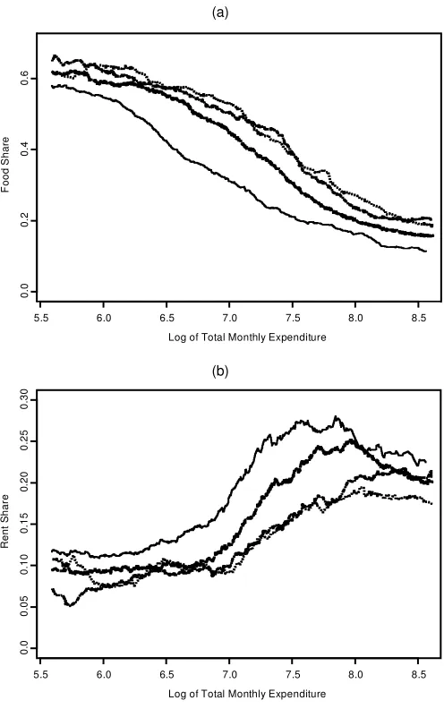
Figure 1(a) portrays Engel curves for food for a selection of family types. As expected, these slope downward, and for a given level of expenditure, food share increases with family

Table 1. Distribution of Family Composition

(Number of Families)

Children

Adults 0 1 2 3 4 5

1 11109 138 126 85 61 14 11533

2 890 526 524 309 144 65 21458

3 373 314 322 233 138 67 11447

4 222 227 230 160 104 66 11009

5 105 117 144 116 66 43 591

6 50 44 71 78 45 32 320

21749 11366 11417 981 558 287 71358

size. Figure 1(b) portrays Engel curves for rent. The rent share is at at low levels of income, then increases before attening out yet again. For a given level of expenditure, rent share generally decreases as family size increases.

As noted by Blackorby and Donaldson (1989, 1993), it is not possible to separately identify the equivalence scale and its elasticity if the share functions are log-linear. A variety

Log of Total Monthly Expenditure

F

o

o

d

S

h

a

re

5.5 6.0 6.5 7.0 7.5 8.0 8.5

0

.0

0

.2

0

.4

0

.6

Log of Total Monthly Expenditure

R

e

n

t

S

h

a

re

5.5 6.0 6.5 7.0 7.5 8.0 8.5

0

.0

0

.0

5

0

.1

0

0

.1

5

0

.2

0

0

.2

5

0

.3

0

(a)

(b)

Figure 1. Engel Curves for (a) Food and (b) Rent. —- Singles; —¢ couples;¢–¢–¢– couples, and one child;¢ ¢ ¢ ¢ ¢ ¢couples, two children.

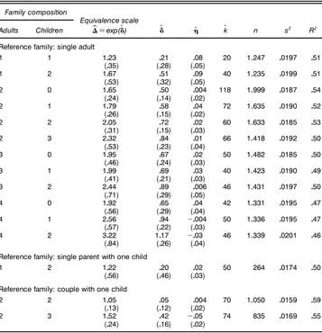
Table 2. Pairwise Estimates of Equivalence Scales, Food Data

Family composition

Equivalence scale

Adults Children bãDexp(ÄO) ÄO ÇO kO n s2 _R2

Reference family: single adult

1 1 1023 021 008 20 11247 00197 051

(035) (028) (005)

1 2 1067 051 009 40 11235 00199 051

(053) (032) (005)

2 0 1065 050 0004 118 11999 00187 054

(024) (014) (002)

2 1 1079 058 004 72 11635 00190 052

(026) (015) (002)

2 2 2005 072 002 60 11633 00185 053

(031) (015) (003)

2 3 2032 084 001 66 11418 00192 050

(053) (023) (004)

3 0 1095 067 002 50 11482 00185 050

(046) (024) (003)

3 1 1099 069 003 40 11423 00190 049

(041) (021) (003)

3 2 2044 089 0006 46 11431 00197 050

(071) (029) (005)

4 0 1092 065 004 42 11331 00195 047

(056) (029) (004)

4 1 2056 094 ƒ0004 50 11336 00195 047

(057) (022) (003)

4 2 3022 1017 ƒ003 46 11339 00201 046

(084) (026) (004)

Reference family: single parent with one child

1 2 1022 020 002 50 264 00174 050

(056) (046) (003)

Reference family: couple with one child

2 2 1005 005 0004 70 11050 00159 059

(013) (012) (002)

2 3 1052 042 ƒ005 74 835 00169 055

(024) (016) (002)

NOTE: Standard errors are in parentheses.

of speciŽcation tests are available in the literature (see, e.g., Yatchew 1998 for references). We use a simple differenc-ing test of speciŽcation against a logarithmic null (Yatchew 1997). We run separate tests for each of the 36 family types in Table 1. Because the null is parametric, undersmoothing the alternative is not necessary. Nevertheless, even for low orders of differencing, the log speciŽcation for the food and rent Engel curves is rejected for most family types. (At mD10, rejection occurs for 30 of 36 family types for the food data and 20 of 36 family types for the rent data.)

Table 2 summarizes estimation results for pairwise compar-isons using the food data. Individually, most estimates of the equivalence scaleãor the log equivalence scaleÄare plausi-ble, although some do not satisfy monotonicity. For example, the estimated equivalence scale for three adults is 1.95, and that for four adults is 1.92. The associated standard errors are large, particularly when considered from a policy standpoint. Furthermore, the “spacings” between estimated equivalence scales are not always plausible and as policy parameters would be difŽcult to defend from an equity standpoint. The explana-tory power is good, withR2_{being around the 50% mark. The} optimalk generally increases with sample size. (For the rent data, theR2_{is typically much lower at around 15%.)}

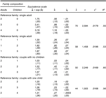
Table 3 summarizes results for the multifamily model (3) applied to four family types at a time using food data. Stan-dard errors are generally smaller than the pairwise estimates in Table 2. In some cases improvements are quite substantial— for instance, the estimated standard error of OÄ for families consisting of four adults and no children improves from .29 to .18. Nevertheless, as a practical matter, the “spacings” again are often implausible, and standard errors remain large. For example, the estimatedãfor a couple with one child relative to a childless couple is 1.03 (standard error .11), that for a couple with two children is 1.52, and that for a couple with three children is 1.57.

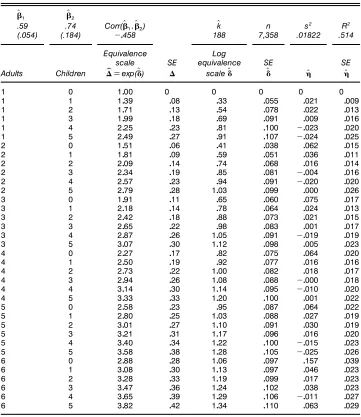
Table 4 presents results for the parsimonious model (5) using food data. The (common) Engel curve is nonparamet-ric, but the equivalence scales satisfy a parametric form that provides for plausible spacings and monotonicity inAandK. Standard errors are much smaller—sometimes by a factor of four—than those corresponding to pairwise or even multifam-ily estimates (Tables 2 and 3). Furthermore, the reduction in explanatory power is modest relative to the completely uncon-strained model (17), which allowsseparate Engel curves for each family type—R2 _{declines from .519 to .514. Applying} test (16), where s2

res is the estimate of the residual variance

from the parsimonious model, we obtain a value of 2.6 for

Table 3. Multifamily Estimates of Equivalence Scales, Food

Family composition

Equivalence scale

Adults Children bãDexp (OÄ) ÄO ÇO Ok n s2 _R2

Reference family: single adult

2 0 1075 056 ƒ001

(020) (012) (002)

3 0 2041 088 ƒ002 _{70 2,594 .0179 .55}

(037) (015) (003)

4 0 3019 1016 ƒ005

(058) (018) (003)

Reference family: single adult

1 1 1030 026 007

(032) (024) (004)

1 2 1082 060 007 _{58 1,458 .0196 .53}

(048) (026) (004)

1 3 1097 068 007

(060) (030) (004)

Reference family: couple with no children

2 1 1003 003 004

(011) (011) (002)

2 2 1052 042 ƒ001 _{50 2,249 .0169 .60}

(017) (011) (002)

2 3 1057 045 ƒ001

(021) (013) (002)

Reference family: couple with one child

2 2 1020 018 ƒ002

(016) (013) (002)

2 3 1026 023 ƒ002 _{44 1,503 .0168 .56}

(019) (015) (002)

2 4 1031 027 ƒ00003

(026) (020) (003)

NOTE: Standard errors are in parentheses.

the (standard normal) test statistic. Although, strictly speaking, this constitutes a rejection, it is not a strong rejection given the sample size and the severity of the constraints. Nor do the comparisons of explanatory power suggest that a grave mis-speciŽcation has been committed. In contrast, the log-linear model, which requires a common slope for all Engel curves but allows separate intercepts for each family type, yields a somewhat lowerR2 _{of .490.}

Overall, given these results, we consider the parsimonious model to be a good compromise. It has desirable monotonicity and spacing properties; yields much more precise estimates than pairwise or multifamily estimation, and with 36 family types, is much easier to compute than the base-independent semiparametric model (3), which imposes no constraints on equivalence scales across family types.

Joint estimation of the two equation parsimonious model yields only very slightly improved estimates when compared to the food equation estimates in Table 4. We obtainÂO1D060 with a standard error of .0538 andÂO2D074 with a standard error of .1788. GLS estimates (see Yatchew et al. 2000 for methodology) were very similar to the joint estimates.

4. EFFICIENCY COMPARISONS

We now discuss the relative asymptotic efŽciency of various speciŽcations. Consider Žrst the single-equation model (3). Because the dummy variables in z are mutually orthogonal,

one might not have expected substantial improvement in preci-sion when estimatingÄusing multifamily data relative to pair-wise estimation. But the beneŽt arises from the fact that under base independence,f is the same for all households. Roughly speaking, the precision of fO depends on the total sample sizen, whereas the precision of household-speciŽc parameters depends directly on the number of observations in that group and indirectly on the precision offO. In the parsimonious spec-iŽcation (5), equivalence scales (4) are a two-parameter func-tion of the number of adults and children, and thus data on all family types are informative in estimation of a particular equivalence scale. For the two-good model (19), becauseÄis common across equations, one would expect improved efŽ-ciency from joint estimation across goods, whether by com-bining single equation estimates using GLS or by performing system estimation.

The cross-equation restrictions should also improve the efŽ-ciency ofÇO₁ and ÇO₂. To see this, refer to (19) and consider the extreme case in which f2 is linear. If one tries to apply single-equation methods to the second equation, then Ä and

Ç2will not be identiŽed separately. But iff1is nonlinear, then

Ämay be identiŽed by applying single-equation estimation to the Žrst equation, then substituting the resultingOÄin the sec-ond equation to produce a consistent estimate ofÇ₂.

To perform efŽciency comparisons, we assume that the data were actually generated by the parsimonious model with parameters set roughly equal to the estimated values; that is,

Table 4. Parsimonious Model Estimates, Food Data

O

Â1 OÂ2

.59 .74 Corr(ÂO11OÂ2) kO n s2 R2

(.054) (.184) ƒ0458 188 7,358 .01822 .514

Equivalence Log

scale SE equivalence SE SE

Adults Children bãDexp(ÄO) ã scaleOÄ OÄ ÇO ÇO

1 0 1000 0 0 0 0 0

1 1 1039 008 033 0055 0021 0009

1 2 1071 013 054 0078 0022 0013

1 3 1099 018 069 0091 0009 0016

1 4 2025 023 081 0100 ƒ0023 0020

1 5 2049 027 091 0107 ƒ0024 0025

2 0 1051 006 041 0038 0062 0015

2 1 1081 009 059 0051 0036 0011

2 2 2009 014 074 0068 0016 0014

2 3 2034 019 085 0081 ƒ0004 0016

2 4 2057 023 094 0091 ƒ0020 0020

2 5 2079 028 1003 0099 0000 0026

3 0 1091 011 065 0060 0075 0017

3 1 2018 014 078 0064 0024 0013

3 2 2042 018 088 0073 0021 0015

3 3 2065 022 098 0083 0001 0017

3 4 2087 026 1005 0091 ƒ0019 0019

3 5 3007 030 1012 0098 0005 0023

4 0 2027 017 082 0075 0064 0020

4 1 2050 019 092 0077 0016 0016

4 2 2073 022 1000 0082 0018 0017

4 3 2094 026 1008 0088 ƒ0000 0018

4 4 3014 030 1014 0095 ƒ0010 0020

4 5 3033 033 1020 0100 0001 0022

5 0 2058 023 095 0087 0064 0022

5 1 2080 025 1003 0088 0027 0019

5 2 3001 027 1010 0091 0030 0019

5 3 3021 031 1017 0096 0016 0020

5 4 3040 034 1022 0100 ƒ0015 0023

5 5 3058 038 1028 0105 ƒ0025 0026

6 0 2088 028 1006 0097 0157 0039

6 1 3008 030 1013 0097 0046 0023

6 2 3028 033 1019 0099 0017 0023

6 3 3047 036 1024 0102 0038 0023

6 4 3065 039 1029 0106 ƒ0011 0027

6 5 3082 042 1034 0110 0063 0029

Â₁D060 andÂ₂D075. We also assume that residuals in the food and rent equations have mean 0 and covariance param-eters Ñ2

1 D00182, Ñ 2

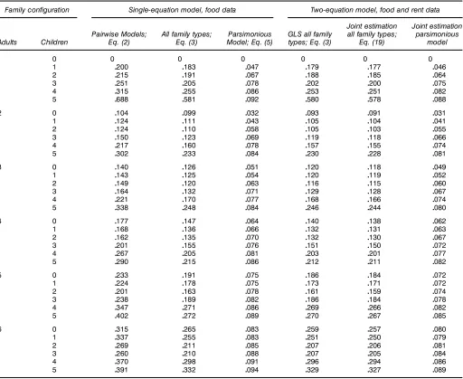
2 D00123, and Ñ12D ƒ00057, and that the distribution of family types and expenditures are Žxed at the values observed in our 7,358 observations. We may now compute the asymptotic standard errors of various estimators (although some would be difŽcult to implement in practice). Table 5 summarizes the results. Consider single-equation esti-mation using food data. As we showed in Table 3, the mul-tifamily speciŽcation (3) can produce signiŽcant efŽciency improvements relative to pairwise estimation even if one esti-mates over relatively small groupings consisting of four fam-ily types. Gains are greatest for those types with fewest data points. Column 4 of Table 5 gives asymptotic standard errors if one were to useall36 family types when estimating model (3) (which would require a grid search in a 35-dimensional space). The gain in efŽciency relative to pairwise estimation can exceed 25% (Table 5, columns 3 and 4). However, the par-simonious model (column 5) yields far greater gains—often a three or four-fold reduction in standard errors (columns 3 and 5).

Turning now to two-equation estimation, estimating equiv-alence scales separately for the food and rent equations using all families in (3) and then applying GLS produces a modest reduction in standard errors, on the order of 2%–3% (Table 5, columns 4 and 6). Joint estimation of both equations using all families [eq. (21)] yields a further improvement of 1%– 2% (columns 6 and 7). Joint estimation of the parsimonious model yields about 1%–2% improvement over estimation of the food equation alone (columns 5 and 8).

In summary, the overwhelming source of efŽciency gains is parsimonious speciŽcation of the equivalence scale as a func-tion of the number of adults and children in the family.

5. CONCLUSIONS

Various methodologies for equivalence scales have been proposed in the literature. Recent examples have been given by Blundell, Preston, and Walker (1994), Citro and Michael (1995), and Van Praag and Warnaar (1997), and in many of the numerous references cited by these authors. Among these methods are subjective approaches, techniques based

Table 5. Relative Ef’ciency of Estimated Equivalence Scales

Family con’guration Single-equation model, food data Two-equation model, food and rent data

Joint estimation Joint estimation Pairwise Models; All family types; Parsimonious GLS all family all family types; parsimonious Adults Children Eq. (2) Eq. (3) Model; Eq. (5) types; Eq. (3) Eq. (19) model

1 0 0 0 0 0 0 0

1 0200 0183 0047 0179 0177 0046

2 0215 0191 0067 0188 0185 0064

3 0251 0205 0078 0202 0200 0075

4 0315 0255 0086 0253 0251 0082

5 0688 0581 0092 0580 0578 0088

2 0 0104 0099 0032 0093 0091 0031

1 0124 0111 0043 0105 0104 0041

2 0124 0110 0058 0105 0103 0055

3 0150 0123 0069 0119 0118 0066

4 0217 0160 0078 0157 0155 0074

5 0302 0233 0084 0230 0228 0081

3 0 0140 0126 0051 0120 0118 0049

1 0143 0125 0054 0120 0119 0052

2 0149 0120 0063 0116 0115 0060

3 0164 0132 0071 0129 0128 0067

4 0221 0170 0077 0168 0166 0074

5 0338 0248 0084 0246 0244 0080

4 0 0177 0147 0064 0140 0138 0062

1 0168 0136 0066 0132 0131 0063

2 0162 0135 0070 0132 0130 0067

3 0201 0155 0076 0151 0150 0072

4 0267 0205 0081 0203 0201 0077

5 0290 0215 0086 0212 0211 0082

5 0 0233 0191 0075 0186 0184 0072

1 0224 0178 0075 0173 0171 0072

2 0201 0163 0078 0161 0159 0074

3 0238 0189 0082 0186 0184 0078

4 0347 0271 0086 0269 0266 0082

5 0402 0272 0089 0270 0267 0085

6 0 0315 0265 0083 0259 0257 0080

1 0337 0255 0083 0251 0250 0079

2 0269 0211 0085 0207 0206 0081

3 0260 0210 0088 0207 0205 0084

4 0370 0298 0091 0296 0294 0086

5 0391 0332 0094 0329 0327 0089

NOTE: For details on multiequation procedures, see Yatchew et al. (2000, appendix).

on assessments of minimum nutritional standards, and utility-based analyses. The latter include Engel and Rothbarth meth-ods, as well as more general demand system approaches. Strong parametric assumptions are usually part of the spec-iŽcation. Pendakur’s generalization allows the calculation of equivalence scales by comparing pairs of nonparametrically estimated Engel curves. We embed Pendakur’s semiparamet-ric speciŽcation in a partial linear index model framework that permits us to simultaneously analyze data on multiple family types. We also propose a parsimonious variant that has further beneŽts. First, because this speciŽcation reduces to two the number of parameters within the index function portion of the model, estimates of equivalence scales are considerably more efŽcient and much easier to compute. This is particularly use-ful when studying data from a developing country, where the number of prevalent family types is often much larger than in data from developed countries. Second, the speciŽcation has the appealing property of being monotone in the number of adults and children, and it yields plausible spacings of equiv-alence scales among families of similar composition. Third,

this framework enables straightforward incorporation of con-tinuous family attributes (such as age) in a parametric way.

These beneŽts are highlighted in our analysis of South African household survey data where our estimated equiva-lence scales are approximately 4AC074K5059_{. Up to a 25%} improvement in efŽciency is achieved when estimating the multifamily model compared with the pairwise model. In con-trast, the parsimonious model yields as much as a four fold increase in precision. Multiple equation estimation (using food and rent data) yields modest gains in precision of less than 5%. In Monte Carlo simulations reported elsewhere (see Yatchew et al. 2000), we Žnd the asymptotically normal approximation of the distribution of coefŽcient estimates [App. eq. (A.7)] to be reasonable at sample sizes over 1,000. We note that estimated standard errors are quite sensitive to selection of the smoothing parameter used to estimate the derivative of the Engel curve. Bootstrap standard errors, although costly to compute, can provide a useful check on those calculated by asymptotic methods.

Finally, we note that many of the estimates of the compo-nents ofÇin the food equations are insigniŽcant or small in magnitude, in which case models (3) and (5) essentially yield Engel’s approach to the estimation of equivalence scales. Per-haps Engel was right after all.

APPENDIX: SINGLE-EQUATION ESTIMATION

Proposition A.1

Consider the model y_iDf 4r 4w_i1Â55Cz_iÇCØ_i, where w_i andz_i are Žnite-dimensional vectors of exogenous variables; f is a nonparametric function;r is a known function; and

Çare Žnite-dimensional parameter vectors;Â₀,Ç₀, andf0are the true parameter values; r0Dr 4w1Â05; and Øi—wi1 zi are

iid with mean 0 and varianceÑ2_{. Set up the model in matrix} notation where theith rows ofW andZarew_i andz_i:

yDf 4r4W 1Â55CZÇCØ0 (A.1)

To estimate this model, proceed analogously to (8)–(10). Fix k. For anyÂ, let PÂ be the permutation matrix that reorders the vectorr 4W 1Â5so that its elements are in increasing order. Apply4IƒS5PÂ to (A.1) to obtain

Here Ok and O will be the values that achieve this minimum, and the estimator ofÇwill beÇO D O‡Â. To obtain large-sample standard errors, deŽne the following conditional covariance matrices:

consistent estimator of the Žrst derivative of f and deŽne

diag4fO0₄

¢55to be the4nƒ Ok5€ndiagonal matrix with diagonal

elementsfO04r 4wi1OÂ55, iD Ok=2C11 : : : 1 nƒ Ok=2, (Ok is even).

DeŽneR to be the matrix whoseith row is the vector partial derivative¡r 4wi1OÂ5=¡Â. Then

1. Proofs of these and multiequation results have been given by Yatchew et al. (2000). They are straightforward vari-ations on existing proofs in the literature, particularly those of Ichimura (1993), Klein and Spady (1993), H¨ardle et al. (1993), and Carroll et al. (1997).

2. In model (3) where separate dummies are permitted for each nonreference family,ÂDÄ1 wD4x1 z51 r4w1Ä5Dlogxƒ

zÄ, andRD ƒZ.

3. In the parsimonious model (5) with separate dummies for each family type entering only in the elasticity term, ÂD

4Â₁1Â₂51 w D4x1 A1 K51 r 4w1Â5DlogxƒÂ₁log4ACÂ₂K5, and the matrixRhasith row

³

This research was supported in part by a grant from the Social Sciences and Humanities Research Council of Canada. The authors are grateful to Gordon Anderson, Dwayne Ben-jamin, Lorne Brandt, Judith Giles, Joel Horowitz, Esfandiar Maasoumi, Angelo Melino, and members of the Canadian Econometrics Study Group for helpful comments. In addition, two referees and an associate editor provided valuable input. Mathew Welch of the University of Cape Town graciously permitted us to post the data.

[Received October 2000. Revised April 2002.]

REFERENCES

Baltagi, B., Hidalgo, J., and Li, Q. (1996), “A Nonparametric Test for Poola-bility Using Panel Data,”Journal of Econometrics, 75, 345–367. Blackorby, C., and Donaldson, D. (1989), “Adult Equivalence Scales,

Interper-sonal Comparisons of Well-Being and Applied Welfare Economics,” Dis-cussion Paper 89-24, University of British Columbia, Dept. of Economics.

(1993), “Adult Equivalence Scales and the Economic Implementation of Interpersonal Comparisons of Well-Being,”Social Choice and Applied Welfare, 10, 335–361.

(1994), “Measuring the Costs of Children: A Theoretical Framework,” inThe Economics of Household Behavior, eds. R. Blundell, I. Preston, and I. Walker, Cambridge, UK: Cambridge University Press, pp. 51–69. Blundell, R., Duncan, A., and Pendakur, K. (1998), “Semiparametric

Esti-mation and Consumer Demand,” Journal of Applied Econometrics, 13, 435–461.

Blundell, R., Preston, I., and Walker, I. (eds.) (1994),The Measurement of Household Welfare, Cambridge, UK: Cambridge University Press. Carroll, R. J., Fan, J., Gijbels, I., and Wand, M. P. (1997), “Generalized

Partially Linear Single Index Models,”Journal of the American Statistical Association, 92, 477–489.

Cavanagh, C., and Sherman, R. (1998), “Rank Estimator for Monotonic Index Models,”Journal of Econometrics, 84, 351–381.

Citro, C., and Michael, R. T. (eds.) (1995), Measuring Poverty—A New Approach, Washington DC: National Academy Press.

Deaton, A. (1997),The Analysis of Household Surveys: A Microeconomic Approach to Development Policy, Baltimore and London: John Hopkins University Press for the World Bank.

Deaton, A., and Muellbauer, J. (1986), “On Measuring Child Costs: With Applications to Poor Countries,” Journal of Political Economy, 94, 720–744.

Fan, Y., and Li, Q. (1996), “Consistent Model SpeciŽcation Tests: Omit-ted Variables and Semiparametric Functional Forms,” Econometrica, 64, 865–890.

Gozalo, P. (1997), “Nonparametric Bootstrap Analysis With Applications to Demographic Effects in Demand Functions,”Journal of Econometrics, 81, 357–393.

Hall, P., Kay, J. W., and Titterington, D. M. (1990), “Asymptotically Optimal Difference-Based Estimation of Variance in Nonparametric Regression,” Biometrika, 77, 521–528.

Hall, P. and A. Yatchew (2002), “Tests of Functional Hypotheses With High Power Against Local Alternatives,” unpublished manuscript, Australian National University, Center for Mathematics and Its Applications. H¨ardle, W. (1990),Applied Nonparametric Regression, Cambridge, UK:

Cam-bridge University Press.

H¨ardle, W., Hall, P., and Ichimura, H. (1993), “Optimal Smoothing in Single-Index Models,”The Annals of Statistics, 21, 157–178.

H¨ardle, W., and Marron, J. S. (1990), “Semiparametric Comparison of Regres-sion Curves,”The Annals of Statistics, 18, 63–89.

(1993), “Comparing Nonparametric versus Parametric Regression Fits,”The Annals of Statistics, 21, 1926–1947.

Horowitz, J., and H¨ardle, W. (1996), “Direct Semiparametric Estimation of Single-Index Models With Discrete Covariates,”Journal of the American Statistical Association, 91, 1632–1640.

Ichimura, H. (1993), “Semiparametric Least Squares (SLS) and Weighted SLS Estimation of Single-Index Models,”Journal of Econometrics, 58, 71–120. Klein, R. W., and Spady, R. H. (1993): “An EfŽcient Semiparametric

Estima-tor for Binary Response Models”Econometrica, 61, 387–421.

Lewbel, A. (1989), “Household Equivalence Scales and Welfare Compar-isons,”Journal of Public Economics, 39, 377–391.

Pendakur, K. (1999), “Semiparametric Estimates and Tests of Base-Independent Equivalence Scales,”Journal of Econometrics, 88, 1–40. Pinkse, C., and Robinson, P. M. (1995), “Pooling Nonparametric Estimates of

Regression Functions With Similar Shape,” inAdvances in Econometrics and Quantitative Economics: Essays in Honor of Professor C. R. Rao, eds. G. S. Maddala, P. C. B. Phillips, and T. N. Srinivasan, Cambridge, MA: Blackwell, 172–195.

Powell, J. L. (1994), “Estimation of Semiparametric Models,” in the Hand-book of Econometrics,(Vol. 4), eds. R. Engle and D. McFadden, Amster-dam: North-Holland, 2443–2521.

Robinson, P. M. (1988), “Root-N-Consistent Semiparametric Regression,” Econometrica, 56, 931–954.

Speckman, P. (1988), “Kernel Smoothing in Partial Linear Models,”Journal of the Royal Statistical Society, B, 50, 413–436.

Van Praag, B. M. S., and Warnaar, M. F. (1997), “The Cost of Children and the Use of Demographic Variables in Consumer Demand,” inHandbook of Population and Family Economics,Vol. 1A, eds. M. R. Rozenzweig and O. Stark, Amsterdam: North Holland, 241–273.

Yatchew, A. J. (1997), “An Elementary Estimator of the Partial Linear Model,” Economics Letters,57, 135–143; additional examples in (1998), Erratum to “An Elementary Estimator of the Partial Linear Model,”Economics Letters, 59, 403–405.

(1998), “Nonparametric Regression Techniques in Economics,” Jour-nal of Economic Literature,36, 669–721.

Yatchew, A. J., and Sun, Y. (2001), “Differencing Versus Smoothing in Nonparametric Regression: Simple Techniques and Monte Carlo Results,” unpublished manuscript, University of Toronto, Dept. of Economics. Yatchew, A. J., Sun,Y., and Deri, C., (2000), “EfŽcient Estimation

of Semiparametric Equivalence Scales With Evidence From South Africa,” working paper, University of Toronto, Dept. of Economics, www.chass.utoronto.ca/¹yatchew/.