www.elsevier.com / locate / econbase
Risk aversion, learning spillovers, and path-dependent economic
growth
*
Randal Verbrugge
Virginia Polytechnic Institute and State University, Blacksburg, VA 24061-6316, USA Received 3 May 1999; accepted 26 January 2000
Abstract
Each agent j[h1, . . . , N receives an independent shock influencing her degree of risk aversion, thenj
undertakes a risky or safe investment. Prior investment in ‘related’ industries reduces the uncertainty. The shock history and this intertemporal interaction determine the long-run growth rate. 2000 Elsevier Science S.A. All rights reserved.
Keywords: Nonergodic; Local interaction; Risk aversion
JEL classification: O4
1. Introduction
One of the puzzling features of cross-country data is that different economies grow at different rates for sustained periods of time; furthermore, early economic development is slow and uncertain (see, e.g., Braudel, 1973; North and Thomas, 1973). On a more local level, agricultural innovations have been observed to spread slowly across regions, so that geographically remote (but observationally similar) regions have employed different agricultural technologies. Part of the cause of slow adoption of new technology is imperfect knowledge about how to implement these innovations, knowledge which in some cases can be gained only from direct experience or learning from the experiences of other plants or firms which use very similar production processes. For example, in the agricultural context, Foster and Rosenzweig (1995) find that imperfect knowledge about how to use new Green Revolution techniques was a significant barrier to their adoption in rural India, and that learning from neighboring farmers’ experiences played a key role in the adoption process.
In this note, I provide a possible explanation for slow and uncertain initial economic development
*Corresponding author. Tel.: 11-540-231-7474; fax:11-540-231-5097.
E-mail address: [email protected] (R. Verbrugge)
and the slow diffusion of new technology (and furthermore demonstrate the possibility of nonergodici-ty, i.e. that some economies might become trapped in low-growth equilibria). The mechanism highlighted, which is reminiscent of that used in Durlauf (1993), relies upon shocks to risk aversion interacting with learning by using spillovers, in the following manner. At the beginning of each time
1
period, each agent receives a shock to her degree of risk aversion, and then must decide between investing in a risky ‘next generation’ project and a safe project. The variability of (or degree of uncertainty about) the agent’s risky project is endogenous, being reduced by previous-period risky
2
investment in this industry and in a (small) group of ‘related’ industries. Thus, risky investment
3
creates an intertemporal informational spillover. The economy is nonergodic: it possesses two distinct long-run steady states.
The posited mechanism is distinct from (but both related to and complementary to) the mechanism described in Acemoglu and Zilibotti (1997) (hereafter AZ). In both frameworks, investment lumpiness, investment return idiosyncracy, and externalities are central. Both feature decisions between safe, low-return projects and risky, high-return projects. AZ explore one extreme: in their set-up, financial relations are essentially costless, and the risk associated with a particular project may be shared by many. However, at a low level of development (wealth), lumpiness means that at most only a few large, risky projects may be embarked upon, and aggregate risk will be high. Increased investment would imply the coverage of more sectors, and hence the reduction of aggregate risk, but small investors ignore the beneficial impact their investment has on reducing the risk facing others, so an inefficiently low number of risky projects are undertaken. The result is slow early development, which is highly variable: a bad draw (the failure of all the risky projects) reduces available capital, leading to low investment next period.
This model starts from the other extreme: financial markets are assumed to be highly incomplete (due, e.g., to prohibitive costs of intermediation or to insurmountable moral hazard problems), so the risks associated with a particular lumpy investment cannot be shared; further, interactions are strictly
4
local in nature — the riskiness of investment in sector j depends only upon past investment in sector j and related sectors, rather than economy-wide prior investment. The key exogenous driving force in
this model is (idiosyncratic) shocks to preferences (rather than last period’s projects’ returns): ‘bad’ preference shocks today will reduce risky investment this period, and this will in turn (ceteris paribus) reduce risky investment next period. This is because risky investment conveys a positive
in-formational externality to future investors; this beneficial risk-reducing effect is ignored by
decision-makers, leading to ‘too little’ risky investment (and hence, growth which is ‘too slow’). As this model
1
This may be thought of literally as a shock to risk aversion (some people are naturally born risk-takers, while others are more cautious), or as a shorthand for shocks to income (e.g. for subsistence farmers, a negative shock to income (or available farmland) is likely to make the agent more risk-averse).
2
For example, agent j might learn from mistakes that his predecessors made, learn about the optimal input mix, deduce the best way to arrange the new equipment, learn about required managerial talent, and so on.
3
Intertemporal investment spillovers have received some degree of attention recently — for example, see Foster and Rosenzweig (1995), Gale (1996), Acemoglu and Scott (1997), Ruiz (1998), and Cooper and Johri (1997) for theory and evidence.
4
highlights the limited or local nature of interaction, it can help describe how innovations may spread across geographical or process-characteristic space over time.
5
This model also features nonergodicity, which is not present in AZ. For example, suppose that, at period t, many agents receive shocks which make them highly risk averse; ceteris paribus, those agents would invest in the safe technology. This increases the risk facing agents at t11, hence tends to diminish future risky investment. A few more bad draws, and the economy could converge to a low-growth equilibrium in which only safe, low return investments are made regardless of future risk
aversion shocks. Conversely, an otherwise identical economy might converge to a high-growth
equilibrium (associated with only risky investments being made), if it happened to receive a different sample path of preference shocks.
2. Model
The economy evolves in discrete time. At every discrete date t, there exist N agents (indexed by i ), each of which is an owner-entrepreneur associated (by birth) with a particular industry; thus industries and agents share the identical index. (Put differently, each industry j is associated with a unique individual (also labeled j ); one could think of each industry j –individual j pair as a distinct ‘family monopoly’.) Agents live for one period, make an investment decision, reproduce, and then pass away, bequeathing their end-of-period capital stock to their (unique) offspring. At every discrete date t, newly born agent i faces a decision between two industry-specific next-generation (date t) technologies (or investment projects), one which is safe (nonstochastic) and the other which is ‘risky’. Agents must select one of these two technologies to allocate all of their existing capital to; financial intermediation is assumed to be prohibitively difficult, so that each agent must bear the entire risk of his decision. During the period, agents live off of a flow of returns generated by their investment. At the end of the period, the investment generates an additional amount of capital (which may be interpreted as ‘new investment’ required to achieve access to the next generation technology). Furthermore, in a learning by using fashion, the act of production creates two potential next-generation investment projects for the next period. Industries interact intertemporally in that previous-period use of the risky technology by industry i and by ‘similar’ industries (defined below) reduces the
variability of the return of i’s next-generation risky technology. Agents cannot draw down their
capital, nor can they sell it, as it is completely industry-specific and has no scrap value. However, capital does not depreciate.
The safe technology, project 1, possesses the production function
y5AKt (1)
where y is output, K is the amount of capital allocated to the project, and A is a positive constant. Att the end of the period, project 1 generates x1 units of capital. The risky technology, project 2, possesses the production function
y5sA1m1´tdKt (2)
5
wherem.0 and´tis a random variable which is distributed normally with mean 0 and with variance
6
described below. Project 2 generates x2.x1 units of capital at the end of the period. Each agent i at date t has the following preferences:
2 2
ui,ts dp 5mp2g si,t p (3)
where p denotes the project identity (1 or 2), mp denotes the expected return of project p, gi,t is a random variable distributed iid (across both agents and time) and uniform [0,1] which dictates the
2
degree of risk aversion, and sp denotes the variance of project p. (Recall that project 1, the safe project, has variance 0).
The variance of i’s project 2 depends upon the previous period’s technology choices by i and by ‘similar’ industries in the following manner. Associated with each agent i is a subset of the N industries, denoted Ne(i ); these will be termed i’s ‘neighbors’. It is assumed that these neighbors possess ‘similar’ technologies, similar in the precise sense that risky investment in these industries provides information about risky investment in i. For this reason, it is assumed that i[Ne(i );i.
Denote the cardinality of Ne(i ) by [Ne(i ). A possible neighborhood structure would associate each
industry with a point on a d-dimensional lattice, and posit ‘neighbors’ to be all industries associated with lattice points a distance 1 away. (However, much more general neighborhood structures are possible — see Verbrugge, 1999.) Denote the number of industries in Ne(i ) which used the risky technology at date (t21) by n2t21, and let n1t21 denote ([Ne(i )2n2t21). Define jit:5(n2t212
This captures the idea that the productivity of the next-generation technology is less uncertain when there has been more experience with the previous generation technology.
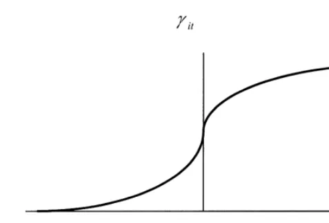
Optimal behavior on the part of agent i can be summarized in Fig. 1. The vertical axis represents
git, the random taste shock. The horizontal axis represents jit, which summarizes the recent behavior of the similar industries (and hence, summarizes the variance of the risky technology). If sjit,gitdlies below the dark curved line, the optimal decision on the part of the agent is to invest in the risky technology. For example, consider the pair 3 / 4, 1 / 2 . Risk aversion is moderate, but the variance ofs d
the risky technology is low, hence it is optimal to choose the risky technology.
Results provided in lemma 2 of Verbrugge (1999), combined with some simple manipulations, prove that this economy is nonergodic and path-dependent: the long run distribution of output (thus, the long run growth rate and variability) depends upon the sample-path realization of taste shocks. The intuition is straightforward, and obvious from Fig. 1. Suppose all agents in the economy happen to invest in the risky technology this period. In that case, next period all agents in the economy will again choose to invest in the risky technology, no matter what their degree of risk aversion — the variance of the risky technology is so low that even the most risk averse find the risky project optimal.
6
One may interpret xi as a (common) fraction of output devoted to investment rather than consumption; the saving decision has been suppressed for simplicity.
7
Fig. 1. Graphical depiction of optimal behavior.
Thus, ‘all play risky’ is an irreducible closed set. Further, as the fraction of agents investing in the risky technology rises above 0.5, further increases in this fraction become more likely. Conversely, suppose all agents in the economy happen to invest in the safe technology. Then, the economy becomes trapped in a low growth state — all agents hereafter will invest in the safe technology, since the variance of the risky technology is so high that even the least risk-averse still find it too risky. (In other words, ‘all play risky’ is also an irreducible closed set.) Further, as the fraction of agents investing in the risky technology falls below 0.5, further decreases in this fraction become more likely.
Though one cannot make strict welfare comparisons (as one long run equilibrium is stochastic, with
8
a wide support), a risk-averse benevolent dictator would select the high-growth equilibrium.
3. Conclusion
This note demonstrates the possibility that learning by using and learning from neighbors, combined with stochastic risk aversion, can lead to slow and uncertain economic development, and to nonergodic (path-dependent) economic growth. Cautious behavior ‘early’ in an economy’s history will result in too little risky investment and can cause the economy to become ‘locked-in’ to safe investments and slow growth. An otherwise identical economy, but one which received a different history of preference shocks, could converge to a high growth equilibrium, in which innovation is rapid and investments are made in riskier technologies which, on average, exhibit higher returns.
Acknowledgements
Thanks are due to Richard Cothren, and also to an anonymous referee, whose comments were extremely useful; however, all errors are mine.
8
References
Acemoglu, D., Scott, A., 1997. Asymmetric business cycles: theory and time-series evidence. Journal of Monetary Economics 40, 501–533.
Acemoglu, D., Zilibotti, F., 1997. Was Prometheus unbound by chance? Risk, diversification, and growth. Journal of Political Economy 105, 709–751.
Braudel, F., 1973. Capitalism and Material Life, 1400–1800, Harper and Row, New York.
Cooper, R., Johri, A., 1997. Dynamic complementarities: a quantitative analysis. Journal of Monetary Economics 40, 97–119.
Durlauf, S., 1993. Nonergodic economic growth. Review of Economic Studies 60, 349–366.
Foster, A., Rosenzweig, M., 1995. Learning by doing and learning from others: human capital and technical change in agriculture. Journal of Political Economy 103, 1176–1209.
Gale, D., 1996. Delay and cycles. Review of Economic Studies 63, 169–198.
North, D., Thomas, R., 1973. The Rise of the Western World: A New Economic History, Cambridge University Press, Cambridge.
Ruiz, J., 1998. Machine Replacement, Network Externalities, and Investment Cycles, Universidad Carlos III de Madrid, Manuscript.