Directory UMM :Data Elmu:jurnal:E:Energy Economics:Vol23.Issue2.2001:

(1)

Effects of changes in residential end-uses

and behavior on aggregate carbon intensity:

comparison of 10 OECD countries for the

period 1970 through 1993

Lorna A. Greening

a,U

, Michael Ting

b

, Thomas J.

Krackler

b

a

Consultant, 7780 Marshall Heights Court, Falls Church, VA 22043, USA

b

Energy & En¨ironmental Di¨ision, Lawrence Berkeley National Laboratory, Berkeley, CA, USA

Abstract

Patterns of the evolution of aggregate carbon intensity from residential end uses show greater variability than other sectors. For some countries in this analysis, this measure exhibits significant decreases, while for other countries this measure exhibits significant increases over the period of analysis. The Adaptive Weighted Divisia rolling base year index specification is applied to carbon emissions from the residential sector for 10 OECD countries for the period 1970᎐1993. Decreases in aggregate carbon intensity for six of the countries range less than 8% to almost 72%, and may be attributed to changes in three different factors. However, for all of the countries, decreases are offset by shifts in end-use structure toward more carbon-intensive activities. These shifts are driven by an increase in the number of households with a corresponding increase in floor space, acquisition of greater numbers of major appliances and by an increase in the ‘other’ energy consumption category.䊚_{2001 Elsevier Science B.V. All rights reserved.}

JEL classification:Q41

Keywords:Residential; Energy use; Carbon dioxide emissions

U

Corresponding author. Tel.:q1-703-761-1373.

Ž .

E-mail address:lgdoon@aol.com L.A. Greening .

(2)

( ) L.A. Greening et al.rEnergy Economics 23 2001 153᎐178

154

1. Introduction

The residential sector uses between 20 and 25% of final energy consumed in the

Ž .

OECD IEA, 1997 . Energy using activities such as space conditioning, water heating, the use of major appliances, and the ‘other’ category, which includes the use small household and personal appliances, account for energy consumption in this sector. Changes in the consumption of final energy for residential purposes vary by country. For example, final energy consumption in Denmark has decreased by 28% or approximately 1.6% per year, while final energy consumption in Japan has increased by 170% or approximately 4.4% per year over the period of analysis

Ž1970᎐1993 . As with transport personal transportation and freight , where energy. Ž .

consumption has been increasing annually at slightly less than 1%, these increases

Ž .

are attributable to changes in behavior Greening et al., 1996, 1998c . These changes in behavior have included increases in population and the numbers of households, an increase in the square footage of the average dwelling, and decreases in the average number of occupants. Along with increased penetration and usage of energy-using technologies, these factors should continue to drive increases in energy consumption for the majority of countries and increases in global carbon emission levels.

More than any other sector, we can directly link changes in residential energy

Ž .

consumption to changes in human activity Schipper et al., 1992 . Analysis of these

1 _Ž _.

changes have been approached by a variety of disciplines Lutzenhiser, 1992 .

However, no single approach has provided an indisputable framework for analysis. For this discussion, we will emphasize the role of economics in determining changes in levels of energy consumption. Under this paradigm, changes in energy prices and income are a primary driver of changes in energy consumption. How-ever, other factors such as climate, household demographics, life-style, culturaliza-tion and governmental policy, also, play a role in determining the choices of types,

Ž

sizes and amounts of energy-using equipment and household living areas Haas,

.

1997 . Using micro-level data, the contribution of these other factors to changes in

Ž .

levels of energy consumption can be evaluated Greening et al., 1998b . However, with aggregate data, we are limited to the observed changes in the average number of dwellings, the average number of occupants, the average square footage of a dwelling, penetration rates of general classes of energy-consuming equipment, and

Ž .

average climate heating and cooling degree days . This severely limits the types of

Ž .

inferences we can draw from the analysis Golove and Schipper, 1997 .

As with the decomposition efforts for other sectors, a primary issue is the identification of the appropriate activity measure to use as a basis for development

1

Those disciplines include energy technologists, whose primary emphasis has been on the role of a given technology without consideration of the factors that lead to adoption, anthropologists, sociologists, psychologists, architects, economists, and others. A good overview of these various lines of approach to

Ž .

(3)

Ž .

of measures of aggregate carbon intensity Greening and Greene, 1998 .

Con-sumers demand energy services, of which energy is only one input.2 Ideally, carbon

emissions should be disaggregated on a per unit basis of energy service. However, unlike either personal transportation or freight, where passenger-kilometers or

Ž .

tonne-kilometers, are routinely measured for different modes activities , residen-tial end uses do not have a similar common measure of activity. For example, in the case of space conditioning, consumers are really demanding thermal comfort. As a measure of thermal comfort, the thermostat set point could be used, or the ambient temperature of the living space. Likewise, for water heating services, the number of gallons of hot water provides an activity measure. However, with the exception of a few isolated, metered studies of an end use, these measures have not been routinely collected. Also, since these measures have different units, different end uses are difficult to combine. Therefore, proxy measures must be determined for each service or end use. To combine them, measures of carbon emissions, structure and energy intensity are usually normalized by population, resulting in

Ž .

per capita measures Schipper et al., 1985 .

Several previous studies have been performed attributing changes of carbon emissions and energy to changes in fuel mix, energy intensity, and activity mix

Žstructure . However, in comparison to either manufacturing or personal.

Ž .

transportation this number is much smaller Greening et al., 1996, 1997, 1998a . This smaller number is the result of the difficulties in obtaining good time series for the relevant data, and then the assignment of energy consumption to various

Ž

end uses Schipper and Ketoff, 1985; Shinbaum and Schipper, 1993; Schipper et al.,

.

1996 . Therefore, valid comparisons between previous studies and our work are difficult, and in some cases impossible. For this discussion of previous decomposi-tion efforts of residential energy and carbon, we will focus on the most

contribu-Ž .

tion to the literature by Schipper et al. 1998 . That work was performed with the same data set, which underlies our analysis, and the same assumptions concerning allocation of energy consumption by end use.

Ž .

Schipper et al. 1998 decomposed carbon emissions from the residential sector for the period 1973 through 1991 for the same 10 OECD countries included in this analysis. Using a Laspeyre’s index specification with a fixed base year, the authors attributed changes in absolute emissions levels to five different factors, including changes in population, changes in primary mix for the generation of electricity, changes in the final fuel mix, changes in energy intensity and changes in structure. Schipper found that structural changes induced by changes in human behavior resulted in increases in levels of carbon emissions. With the exception of Norway, structural shifts towards more carbon-intensive activities resulted in increases of carbon emissions of between 15 and 65%. These shifts in structure partially offset the reductions in emissions levels achieved through decreases in energy intensity

2

Energy services are produced by the use of fuel, capital, labor and management expertise by

Ž .

(4)

156

Ž17᎐41% for nine of the countries . These two terms are most comparable with the.

analysis presented here, and patterns of change for both terms for each of the countries are the same between the two studies. However, the magnitudes vary as a result of the specification of five terms and the indexing method used.

The work presented here analyzes development of carbon emission trends from residential energy consumption in 10 OECD countries: Denmark, Finland, France,

Ž .

Germany West , Italy, Japan, Norway, Sweden, the UK, and the US. Decomposi-tion of aggregate carbon intensity allows attribuDecomposi-tion of changes in this measure to changes in the primary fuel mix for the generation of electricity, changes in final fuel mix for all residential end uses, and changes in energy intensity and end use

Žactivity mix structure. As with our previous analyses of sectoral emissions trends,.

we use a modified Adaptive Weighting Divisia index specification. As with our other sectoral studies, declines in energy intensity made a substantial contribution to declines in residential carbon intensity in the majority of countries in this analysis. In addition, declines in aggregate carbon measures also result from significant shifts towards a less carbon-intensive mix for both primary fuels used in the generation of electricity and final fuels. However, for the majority of countries, shifts in the activity mix or structure of end uses offset either partially or totally those declines in aggregate carbon intensity resulting from changes in these other measures. As a result, cumulative changes in per capita carbon emissions, our measure of aggregate carbon intensity, show a great deal of variability. Six of the countries exhibit declines ranging from almost 8% for the US to almost 72% for Sweden. The other four countries exhibit increases of less than 1% to well over 94%.

The remainder of this paper is organized into several sections. Section 2 provides an overview of the parametric framework for the carbon decomposition index and discusses the data used in the analysis. The complete technical development of the index decomposition method is presented in Appendix A. Section 3 of the main body of the text discusses the results of our analysis. The final section provides brief concluding remarks.

2. Specification of the index decomposition method and data

A modified or rolling base year specification of the Adaptive Weighting Divisia

ŽAWD Index method is used to decompose and attribute changes in aggregate.

carbon intensity to several different factors. This method has been previously used to decompose sectoral aggregate carbon for manufacturing, freight and personal

Ž .

transportation Greening et al., 1996, 1998a,c . In comparison to other index decomposition methods, this indexing method is more robust, exhibiting a smaller

Ž .

(5)

2.1. Methods of decomposition

Aggregate carbon intensity may be expressed by a multiplicative relationship, and for residential end uses, changes in aggregate carbon may be attributed to four different factors. For a four-term index decomposition, changes in the aggregate carbon intensity index may be attributed to changes in the primary fuel mix used for electricity generation, changes in the final fuel mix, changes in energy intensity and changes in the structure or mix of residential energy services consumed. This relationship can be expressed as follows:

Ž1q⌬%G_tot.sŽ1q⌬%G_emissions. Ž₎ 1q⌬%G_fuel. Ž₎ 1q⌬%G_intensity.

Ž . Ž .

) 1q⌬%Gend-use ) 1qD

Ž .

where D is the unexplained residual or approximation error represented by the

quotient of the product of the four terms on the right hand side and the actual change in aggregate carbon intensity.

The AWD provides more robust estimates of changes in aggregate carbon intensity by reconciling the results from a discrete and a continuous index decom-position method. The reconciliation process is performed through the application of a weighting scheme to the difference between the current year and the base year of the various factors of attribution. The weighting scheme is derived through

Ž

equating the two end points of a parametric family of indices Liu et al., 1992;

. Ž .

Greening et al., 1997 . The end points are defined by a discrete Laspeyre’s index

Ž .

decomposition method, and a continuous simple Divisia index decomposition

Ž .

method Greening et al., 1997 . Each of these end points provides for different assumptions concerning the path of integration, and as such, the results of each method will be slightly different. The weights defining the value of the index between the two end points change from year to year as emissions, energy consumption, and various other measures change. The technical derivation of the AWD and the weighting scheme is provided in Appendix A. Table A-1 provides the variable and notational definitions for that development.

2.2. Data

Data for this analysis was taken from files maintained at Lawrence Berkeley National Laboratory. Time series of final energy consumption by fuel type, primary energy consumption by fuel type used for electricity generation, population, the number of households, energy consumption by major residential end-use, the number of square meters of housing and the number of major house appliances were used in this analysis. These series were collected from a variety of official or industry sources, including energy companies, utilities, appliance manufacturers

Ž .

(6)

158

methods and differences between data sources,3 efforts have been made to

recon-cile those data sources, and missing values have been interpolated. Allocations of end-use energy consumption are made on the basis of observed relationships between an activity and energy consumption from survey data or similar

instru-ments.4 For space conditioning, energy consumption has been normalized for the

number of heating degree days.5 As a result of these modifications to the data,

particularly for the countries6 of Finland, France and Italy, interpretation of

results, especially the inference of long-term trends, must be done with care. To avoid some of the potential for misinterpretation of results, we have adopted the practice of reporting period averages as a means of smoothing out some these discrepancies.

Available carbon emissions were estimated using the latest methods

recom-Ž .

mended by the Intergovernmental Panel on Climate Change IPCC, 1995 . The carbon emissions factors used by the IPCC are the result of recent contributions to the literature in this area and for most fuels are slightly higher than previously published results. However, our estimates of aggregate carbon do not reflect the

Ž .

effects of other greenhouse gases GHG , e.g. nitrogen oxides, which may have a

Ž .

greater radiative forcing effect on the atmosphere Shine et al., 1990 . Estimates of other GHG emissions from residential energy consumption require a number of additional assumptions on combustion efficiencies and the types of combustion technologies in use. These types of assumptions cannot be made with aggregate data. As a result this analysis is restricted to examining changes in the rates of growth of available carbon.

Available carbon estimates by sector are developed using fuel specific carbon coefficients and adjusting for the heating value of each fuel across countries. To allow for incomplete combustion, only 99% of available carbon is assumed com-busted. Waste biomass fuels, which may be a substantial energy source in the generation of electricity, are assigned an emissions factor of zero based on the assumption that the carbon released from combustion of this source is equivalent to the carbon sequestered by biomass replacement. Since electricity is a major final energy source for residential consumption, and the primary energy types used in

Ž

electrical generation have been shifting from solid to other fuel types natural gas,

.

nuclear, biomass and hydro , carbon coefficients for electricity were calculated based on primary energy shares for each year of the time period under evaluation.

3

For the countries Finland, Sweden and Denmark, data must be combined from several sources

ŽIEA, 1997 ..

4

Allocation of energy consumed for each end use is based primarily on survey data, and converted to

Ž . Ž .

unit energy consumption values UEC Schipper et al., 1985 . 5

The energy consumption for space heating has been weather normalized by multiplying it by the inverse of the percentage deviation of that year’s degree-days from the long-term average. The cut-off

Ž .

varies with the country, depending upon climate IEA, 1997 . 6

Of the countries included in this analysis, the national authorities of these countries do not publish

Ž .

(7)

This procedure captures not only changes in fuel mix, but also changes in generation technologies and capacity utilization, and improvements in generation efficiencies.

Similar assumptions were not made for the emissions coefficients of other primary fuels. The carbon emissions coefficients for these fuels were held constant over the entire period of analysis. We must acknowledge that emissions for other primary fuels have changed over time due to changes in grades of fuel, however, these changes are expected to be small and data allowing for evaluation of such changes are not available. This simplification means that the emissions index term,

Ri jt, which in the broader methodological framework would capture changes in

emissions from other fuels, is restricted to only changes in emissions from electrical generation.

3. Discussion of results

Tables 1᎐6 present the results for all of the countries in this analysis of

residential energy consumption. Table 1 provides the cumulative results for the AWD decomposition of aggregate carbon intensity. Table 2 presents estimates of

Ž

elasticities of some of the key variables energy consumption, aggregate carbon

.

intensity, carbon emissions and energy intensity with respect to a consumption

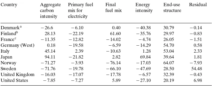
Table 1

Cumulative percent changes in aggregate carbon intensity, primary fuel mix for electricity generation, final fuel mix, energy intensity, end-use structure, and residual terms of the decomposition of carbon

Ž

emissions from residential for 10 OECD countries for the period 1970᎐1993 shown in total percent

.

change from 1970

Country Aggregate Primary fuel Final Energy End-use Residual

carbon mix for fuel mix intensity structure intensity electricity

a

Denmark y26.6 y6.10 0.40 y40.38 30.79 y0.14

b

Finland 28.13 y22.19 61.60 y35.76 29.97 y0.83

c

France y11.35 y12.82 y14.02 y4.74 26.05 y1.51

Ž .

Germany West 0.18 y19.58 y6.59 y14.29 54.70 0.58

Italy 45.14 2.39 y10.63 1.28 53.04 2.33

Japan 94.11 y21.82 2.82 69.84 39.64 1.81

Norway y71.27 y3.93 y76.14 y17.03 64.07 y7.93

Sweden y71.76 y19.78 y66.10 y47.69 28.50 54.48

United Kingdom y16.03 y17.07 y17.78 y6.57 32.39 y0.43

United States y7.85 y7.27 5.89 y27.10 20.19 6.98

a

Data for Denmark were only available after 1972; total period of analysis reflects 1972᎐1993. b

Data for Finland and the UK were only available between 1970 and 1992; total period of analysis reflects 1970᎐1992.

c

(8)

()

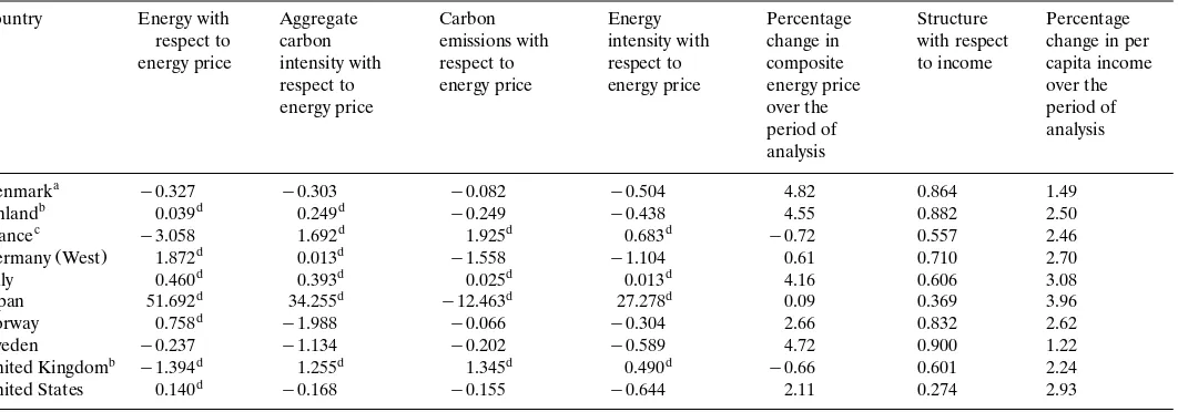
Elasticities with respect to the own-price energy of energy, aggregate carbon intensity, carbon emissions, energy intensity, percentage change in composite energy price, elasticity of structure with respect to income, and percentage change in per capita household expenditures as a proxy for household income

Country Energy with Aggregate Carbon Energy Percentage Structure Percentage

respect to carbon emissions with intensity with change in with respect change in per energy price intensity with respect to respect to composite to income capita income

respect to energy price energy price energy price over the

energy price over the period of

period of analysis

analysis a

Denmark y0.327 y0.303 y0.082 y0.504 4.82 0.864 1.49

b d d

Finland 0.039 0.249 y0.249 y0.438 4.55 0.882 2.50

c d d d

France y3.058 1.692 1.925 0.683 y0.72 0.557 2.46

d d

Ž .

Germany West 1.872 0.013 y1.558 y1.104 0.61 0.710 2.70

d d d d

Italy 0.460 0.393 0.025 0.013 4.16 0.606 3.08

d d d d

Japan 51.692 34.255 y12.463 27.278 0.09 0.369 3.96

d

Norway 0.758 y1.988 y0.066 y0.304 2.66 0.832 2.62

Sweden y0.237 y1.134 y0.202 y0.589 4.72 0.900 1.22

b d d d d

United Kingdom y1.394 1.255 1.345 0.490 y0.66 0.601 2.24

d

United States 0.140 y0.168 y0.155 y0.644 2.11 0.274 2.93

a

Data for Finland and the UK were only available between 1970 and 1992; total period of analysis reflects 1970᎐1992. c

Data for France were only available between 1975 and 1992, total period of analysis reflects 1975᎐1992. d

(9)

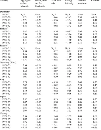
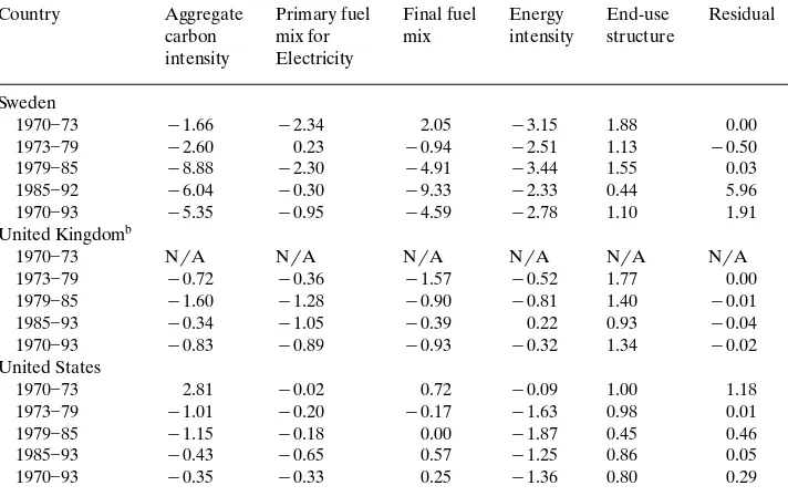
Table 3

Geometric mean of changes in the aggregate carbon intensity, primary fuel mix for electricity generation, final fuel mix, energy intensity, end-use structure, and residual terms of the decomposition of carbon emissions from residential energy consumption for 10 OECD countries for the period

Ž .

1970᎐1993 shown in percent per annum

Country Aggregate Primary fuel Final fuel Energy End-use Residual

carbon mix for mix intensity structure

intensity Electricity a

Denmark

1970᎐72 NrA NrA NrA NrA NrA NrA

1972᎐79 0.71 0.30 0.64 y2.42 2.35 y0.09

1979᎐85 y2.71 y0.28 y0.26 y3.34 1.09 0.11

1985᎐93 y2.40 y0.83 y0.31 y1.76 0.51 y0.02

1972᎐93 y1.46 y0.30 0.02 y2.43 1.29 y0.01

b Finland

1970᎐73 6.87 y0.05 4.76 y0.87 2.95 0.01

1973᎐79 2.96 0.39 3.48 y3.14 2.30 0.02

1979᎐85 y0.44 y3.06 2.30 y1.50 2.08 y0.16

1985᎐93 y1.41 y1.22 y0.01 y1.90 1.76 y0.01

1972᎐93 1.13 y1.13 2.21 y1.99 2.16 y0.04

c France

1975᎐79 1.50 y0.46 0.22 y0.21 1.97 y0.01

1979᎐85 y1.56 y1.10 y3.04 1.20 1.41 0.04

1985᎐92 y1.22 y0.74 0.36 y1.59 1.00 y0.24

1972᎐92 y0.71 y0.80 y0.88 y0.29 1.37 y0.09

Ž .

Germany West

1970᎐73 2.30 y0.64 y0.81 0.08 3.51 0.19

1973᎐79 0.88 y1.03 y0.02 y0.94 2.92 0.00

1979᎐85 y1.63 y1.27 y0.07 y2.03 1.76 0.01

1985᎐93 y0.26 y0.75 y0.48 0.29 0.70 y0.01

1972᎐93 0.01 y0.94 y0.30 y0.67 1.92 0.03

Italy

1970᎐73 5.75 0.73 y0.58 2.23 3.05 0.23

1973᎐79 2.02 0.11 y0.02 y0.42 2.20 0.15

1979᎐85 y0.04 y0.03 y0.46 y1.21 1.62 0.05

1985᎐93 1.10 y0.04 y0.82 0.56 1.36 0.05

1970᎐93 1.63 0.10 y0.49 0.06 1.87 0.10

Japan

1970᎐73 7.52 y0.50 0.13 5.67 1.89 0.23

1973᎐79 4.07 y1.15 0.38 3.00 1.86 y0.03

1979᎐85 y0.32 y1.79 0.04 0.33 1.08 0.03

1985᎐93 2.86 y0.67 y0.02 2.11 1.29 0.14

1972᎐93 2.93 y1.06 0.12 2.33 1.46 0.08

Norway

1970᎐73 2.56 y0.47 1.48 y2.39 4.04 0.00

1973᎐79 y4.02 y0.06 y5.40 y0.56 2.15 y0.06

1979᎐85 y7.76 0.29 y8.55 y1.96 2.56 0.03

1985᎐93 y7.13 y0.49 y7.31 0.49 1.22 y1.00

(10)

162

Ž .

Table 3 Continued

Country Aggregate Primary fuel Final fuel Energy End-use Residual

carbon mix for mix intensity structure

intensity Electricity Sweden

1970᎐73 y1.66 y2.34 2.05 y3.15 1.88 0.00

1973᎐79 y2.60 0.23 y0.94 y2.51 1.13 y0.50

1979᎐85 y8.88 y2.30 y4.91 y3.44 1.55 0.03

1985᎐92 y6.04 y0.30 y9.33 y2.33 0.44 5.96

1970᎐93 y5.35 y0.95 y4.59 y2.78 1.10 1.91

b United Kingdom

1973᎐79 y0.72 y0.36 y1.57 y0.52 1.77 0.00

1979᎐85 y1.60 y1.28 y0.90 y0.81 1.40 y0.01

1985᎐93 y0.34 y1.05 y0.39 0.22 0.93 y0.04

1970᎐93 y0.83 y0.89 y0.93 y0.32 1.34 y0.02

United States

1970᎐73 2.81 y0.02 0.72 y0.09 1.00 1.18

1973᎐79 y1.01 y0.20 y0.17 y1.63 0.98 0.01

1979᎐85 y1.15 y0.18 0.00 y1.87 0.45 0.46

1985᎐93 y0.43 y0.65 0.57 y1.25 0.86 0.05

1970᎐93 y0.35 y0.33 0.25 y1.36 0.80 0.29

a

c

Data for France were only available between 1975 and 1992, total period of analysis reflects 1975᎐1992.

weighted, composite price of residential energy, and structure with respect to

Ž .

income average household expenditures are used as a proxy for this variable . This allows evaluation of the role of price and income in determining the changes in these variables over the period of analysis. Table 3 presents the geometric means of the growth rates of aggregate carbon intensity and each of the index terms of

our aggregate carbon decomposition. Tables 4᎐6 present the end-use shares of

final energy consumption for the residential sector, the fuel shares of final energy consumption, and the fuel shares for primary energy used in the generation of electricity.

Four periods of time are used to present the results on Tables 3᎐6. These four

periods were chosen to correspond to four different periods in world energy

Ž .

markets: 1 1970 through 1973, a period of relatively low energy prices just prior to

Ž .

the first oil embargo; 2 a period of generally increasing energy prices from 1973

Ž .

through 1979; 3 1979 through 1985, a period of even higher energy prices after

Ž .

(11)

Table 4

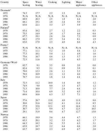
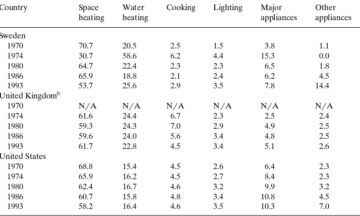
End-use shares for residential final energy consumption in 10 OECD countries over the period 1970᎐1993

Country Space Water Cooking Lighting Major Other

heating heating appliances appliances

a Denmark

1972 74.3 17.7 2.2 1.3 2.6 1.9

1974 NrA NrA NrA NrA NrA NrA

1980 68.9 20.3 2.5 1.8 4.4 2.0

1975 77.1 11.1 5.2 1.0 4.4 1.2

another. The effect, however, varied with the end use Greening et al., 1996,

.

(12)

164

Ž .

Table 4 Continued

Country Space Water Cooking Lighting Major Other

heating heating appliances appliances

1974 61.6 24.4 6.7 2.3 2.5 2.4

c

Data for France were only available between 1975 and 1992, total period of analysis reflects 1975᎐1992.

Examination of our results indicates that residential consumers in countries, where aggregate carbon intensity declined over the analysis period, do have some sensitivity to changes in energy prices. However, this relationship is not universal. Since the residential sector has been the target of a number of conservation programs during the period of analysis, declines in energy consumption may also be attributed to those programs. Disentangling declines in energy consumption or emissions levels as a result of those programs from price-induced declines is not possible with the aggregate data used in this analysis. Generally, however, increases

Ž

in energy prices do appear to somewhat retard increases in emissions and energy

.

consumption , and promote improvements in energy intensity, i.e. energy intensity declines in response to increases in energy price. For all of the countries the income effect, as demonstrated by changes in structure and the elasticity of this variable with respect to changes in income, appears to outweigh the effects of energy prices. However, as per capita income increases across our sample of countries, increases in emissions resulting from a shift in structure decline. Gener-ally, consumers in countries with the greatest increases in per capita income over

Ž .

(13)

Table 5

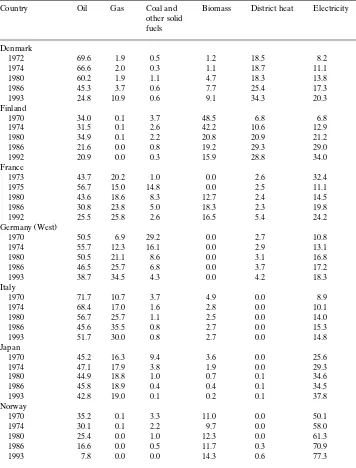
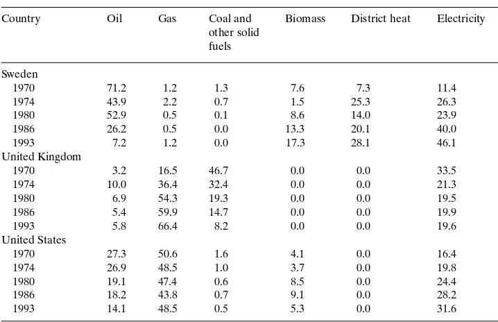
Fuel shares of final energy use by the residential sector in 10 OECD countries over the period

Ž .

1970᎐1993 percent of total final energy

Country Oil Gas Coal and Biomass District heat Electricity

other solid fuels Denmark

1972 69.6 1.9 0.5 1.2 18.5 8.2

1974 66.6 2.0 0.3 1.1 18.7 11.1

1980 60.2 1.9 1.1 4.7 18.3 13.8

1986 45.3 3.7 0.6 7.7 25.4 17.3

1993 24.8 10.9 0.6 9.1 34.3 20.3

Finland

1970 34.0 0.1 3.7 48.5 6.8 6.8

1974 31.5 0.1 2.6 42.2 10.6 12.9

1980 34.9 0.1 2.2 20.8 20.9 21.2

1986 21.6 0.0 0.8 19.2 29.3 29.0

1992 20.9 0.0 0.3 15.9 28.8 34.0

France

1973 43.7 20.2 1.0 0.0 2.6 32.4

1975 56.7 15.0 14.8 0.0 2.5 11.1

1980 43.6 18.6 8.3 12.7 2.4 14.5

1986 30.8 23.8 5.0 18.3 2.3 19.8

1992 25.5 25.8 2.6 16.5 5.4 24.2

Ž .

Germany West

1970 50.5 6.9 29.2 0.0 2.7 10.8

1974 55.7 12.3 16.1 0.0 2.9 13.1

1980 50.5 21.1 8.6 0.0 3.1 16.8

1986 46.5 25.7 6.8 0.0 3.7 17.2

1993 38.7 34.5 4.3 0.0 4.2 18.3

Italy

1970 71.7 10.7 3.7 4.9 0.0 8.9

1974 68.4 17.0 1.6 2.8 0.0 10.1

1980 56.7 25.7 1.1 2.5 0.0 14.0

1986 45.6 35.5 0.8 2.7 0.0 15.3

1993 51.7 30.0 0.8 2.7 0.0 14.8

Japan

1970 45.2 16.3 9.4 3.6 0.0 25.6

1974 47.1 17.9 3.8 1.9 0.0 29.3

1980 44.9 18.8 1.0 0.7 0.1 34.6

1986 45.8 18.9 0.4 0.4 0.1 34.5

1993 42.8 19.0 0.1 0.2 0.1 37.8

Norway

1970 35.2 0.1 3.3 11.0 0.0 50.1

1974 30.1 0.1 2.2 9.7 0.0 58.0

1980 25.4 0.0 1.0 12.3 0.0 61.3

1986 16.6 0.0 0.5 11.7 0.3 70.9

(14)

166

Ž .

Table 5 Continued

Country Oil Gas Coal and Biomass District heat Electricity

other solid fuels Sweden

1970 71.2 1.2 1.3 7.6 7.3 11.4

1974 43.9 2.2 0.7 1.5 25.3 26.3

1980 52.9 0.5 0.1 8.6 14.0 23.9

1986 26.2 0.5 0.0 13.3 20.1 40.0

1993 7.2 1.2 0.0 17.3 28.1 46.1

United Kingdom

1970 3.2 16.5 46.7 0.0 0.0 33.5

1974 10.0 36.4 32.4 0.0 0.0 21.3

1980 6.9 54.3 19.3 0.0 0.0 19.5

1986 5.4 59.9 14.7 0.0 0.0 19.9

1993 5.8 66.4 8.2 0.0 0.0 19.6

United States

1970 27.3 50.6 1.6 4.1 0.0 16.4

1974 26.9 48.5 1.0 3.7 0.0 19.8

1980 19.1 47.4 0.6 8.5 0.0 24.4

1986 18.2 43.8 0.7 9.1 0.0 28.2

1993 14.1 48.5 0.5 5.3 0.0 31.6

consumed, and this provides partial support for the concept that energy

consump-7_Ž _.

tion is ‘quasi-homothetic’ Greening and Greene, 1998 .

3.1. Comparison across countries of cumulati¨e changes

Table 1 presents the cumulative results of our analysis across the entire period of analysis. Unlike aggregate carbon measures for other end uses, this measure for residential energy consumption exhibits greater variability. The greatest reductions in aggregate carbon intensity were observed for Sweden, Norway and Denmark, where the declines ranged from over 71% to over 26%. The greatest increases occurred in Japan, Italy and Finland, where increases ranged from slightly over

Ž

94% to slightly over 28%. The other four countries France, West Germany, the

.

UK and the US exhibit levels of change, either increases or decreases, without this degree of variability.

The sources of declines or increases in aggregate carbon intensity can be attributed to one of four factors, which vary in relative importance across the 10

7

The majority of consumer demand models for fuel assume homothetic preferences, i.e. doubling the

Ž .

(15)

OECD countries. For Sweden and Norway, shifts towards less-carbon intensive final fuel mixes and primary fuel mixes for the generation of electricity, provided

Table 6

Ž

Fuel shares for electricity generation in 10 OECD countries over the period 1970᎐1993 percent of total a

.

primary inputs

Country Oil Gas Coal Biomass Nuclear Hydro Other

(16)

168

Ž .

Table 6 Continued

Country Oil Gas Coal Biomass Nuclear Hydro Other

renewables Sweden

1970 51.1 0.0 1.0 0.0 0.2 47.6 0.0

1974 33.3 0.0 1.0 0.1 6.4 59.1 0.0

1980 19.0 0.0 0.2 0.0 46.8 34.4 0.0

1986 1.6 0.3 0.8 0.0 76.2 21.9 0.0

1993 0.9 0.5 0.9 y0.7 70.2 28.2 0.0

United Kingdom

1970 21.1 0.3 67.6 0.0 10.4 0.6 0.0

1974 26.7 3.6 56.7 0.0 12.5 0.5 0.0

1980 11.2 0.8 73.7 0.0 13.8 0.5 0.0

1986 10.4 0.7 66.7 0.0 21.7 0.6 0.0

1993 6.2 9.2 51.3 0.0 32.8 0.5 0.0

United States

1970 13.9 26.2 51.7 0.0 1.8 6.2 0.1

1974 18.0 18.1 50.1 0.0 7.3 6.0 0.5

1980 11.3 15.8 54.6 0.0 13.0 4.5 0.9

1986 5.7 9.9 59.1 0.1 19.4 4.3 1.6

1993 3.5 8.7 56.1 1.6 24.4 3.5 2.3

a

Due to differences in accounting for self or auto production of electricity generated from renewables among countries, fuel shares for this purpose may actually vary slightly from values reported here.

substantial contributions toward the decline in aggregate carbon intensity. In addition for Sweden, declines attributable to decreases of nearly 50% in energy intensity further contributed. Similarly, decreases of slightly over 17% in energy intensity re-enforced the declines in aggregate carbon intensity for Norway. How-ever, shifts towards a more carbon-intensive activity mix in both countries offset the declines attributable to the other factors. For Denmark, a decrease of over 40% in energy intensity provided the majority of the decline in carbon intensity. This decline was also largely offset by shifts toward a more carbon-intensive activity mix.

As with the sources of declines in aggregate carbon intensity, the sources of increases in aggregate carbon intensity for Japan, Italy and Finland are attributed to different sources. For Japan, the largest contributor to increases in aggregate carbon intensity was a nearly 70% increase in energy intensity, which was re-en-forced by a shift towards a more carbon-intensive activity mix or end-use structure of nearly 40%. Increases in energy intensity in Japan are largely the result of

Ž .

(17)

fuel mix, which was once again re-enforced by an almost 30% shift towards a more carbon-intensive activity mix.

The remaining countries of France, West Germany, the UK and the US also exhibit a variety of sources of decreases and increases in aggregate carbon intensity. For all four countries decreases in aggregate carbon intensity resulted from shifts towards a less-carbon intensive primary fuel mix for the generation of electricity, and towards a less carbon-intensive final fuel mix. These shifts were re-enforced by declines in energy intensity. However, for all of these countries, shifts towards a more carbon-intensive activity mix substantially offset these declines.

3.2. Effects of changes in energy prices on carbon emissions, aggregate carbon intensity, and energy intensity

As with our previous analyses of carbon emissions from other end uses, we are interested in the effects of energy prices on moderating growth rates of energy consumption, carbon emissions, and aggregate carbon intensity, while promoting decreases in energy intensity. Tables 2 and 3 provide two different means of examining changes in these factors in response to energy prices. Table 2 provides own-price elasticities with respect to a composite energy price for energy consump-tion, aggregate carbon intensity, carbon emissions, and energy intensity. The percentage change of price over the forecast horizon is also included. The 10% significance level of the elasticity estimates of own-price and structure with respect to income are also noted. Table 3 provides the values for each of the factors of attribution for our four pricing periods, and for the period of analysis in its entirety.

Although increases in energy prices are assumed to result in decreases in energy consumption and carbon emissions, this relationship is not clearly demonstrated by

Ž

our results. For five of the countries Denmark, Finland, Norway, Sweden, and the

.

US there does appear to be a correlation between increases in energy prices and decreases in some of the relevant measures. However, this relationship is not uniform with respect to all of the variables, and this may be the result of the data, or other factors, which could not be controlled for. With the exception of Italy, price increases of over 2% over the period of analysis, resulted in at least a 0.06% decline in carbon emissions for every 1% increase in price. Across countries this relationship varied, and is reflective of the types of energy-using technologies implemented, climate and other factors.

Examination of Table 3 indicates that periods of high price do have some role in promoting declines in aggregate carbon intensity. The price effects in promoting energy intensity do not appear as pronounced as they are for both manufacturing

Ž .

and personal transportation Greening et al., 1996, 1998a . Only six of the coun-tries exhibit increases in the rate of decline in aggregate carbon intensity from that source during periods of higher energy prices. Furthermore, half of the countries

(18)

170

Ž .

intensity during the period of lower prices 1985᎐1993 . This appears to counter

some of the arguments concerning the irreversibility of efficiency improvements

ŽHaas and Schipper, 1998 . These increases though in energy intensity may actually.

reflect the introduction of larger appliances with more energy-consuming features into the energy stock. Aggregate data do not allow us to identify that type of change, and control for it. Only through the use micro-level data, with extensive detail concerning an individual household’s appliance stock over a period of time, allows for this type of analysis.

Decreases in aggregate carbon intensity, also, occur as a result of shifts towards less carbon-intensive mixes for primary fuels for the generation of electricity and

Ž . Ž

delivered final energy fuels. During periods of high energy prices 1973᎐1979, and

.

1979᎐1985 , these shifts were most pronounced for Finland, France, Germany

ŽWest , Japan, Norway, Sweden, and the UK. In the case of France, Norway,.

Sweden and the UK, these shifts towards a less carbon-intensive fuel mix, along with reductions in energy intensity, resulted in reductions in aggregate carbon intensity.

3.3. Effects of changes in income on acti¨ity mix or structure

For all of the countries in this analysis, aggregate carbon intensity increased as a

Ž .

result of shifts towards a more carbon-intensive activity mix Table 1 . Table 2 indicates that a 1% increase in income resulted in between an approximately 0.2% to a 0.9% increase in aggregate carbon intensity as a result of shifts towards a more carbon-intensive activity mix. However, the magnitude of those shifts generally declined with an increase in the percentage change in income over the period of analysis, i.e. generally, the greater the change in income the smaller the resulting shift in activity mix. Examination of Table 3 indicates that during periods of high energy prices, structural shifts towards more carbon-intensive activity mixes de-clined in every country. However, these shifts still occurred.

Table 4 provides an overview of the mix of residential end-use activities at various points in time. The share of energy consumption for space heating consistently declined through time for the majority of countries. However, the rate of decline of energy consumption for this end use varies across countries as a result of the penetration rate of central heating. Central heating utilizes more energy, and as this form of heating increases the share of energy consumption for space

Ž .

heating will increase assuming no decreases in energy intensity IEA, 1997 . However, during the period of analysis, increases in energy consumption for this end use were often offset by improvements in insulation or the implementation of

various other energy conservation measures for building shells.8 The shares of

energy consumption for water heating, and cooking remained either relatively

8

A number of countries during the period of analysis implemented more stringent building codes,

Ž .

(19)

constant or declined across all of the countries. The share of energy consumption for lighting in all countries has increased. This is reflective of an increase in the

Ž .

average square footage of dwellings in these countries IEA, 1997 . Similarly, the share of energy consumption for major appliances has increased over the period of analysis. This is the result of increased penetration of appliances, such as clothes washers, dryers and refrigerators with freezers.

Perhaps, the most interesting change, and possibly predictive of future energy consumption trends in the residential sector, is the increase in the consumption of energy in the ‘other’ category. Increases in all of the countries ranging from 1%

ŽDenmark to 13% Sweden for this category are indicated. Whereas, other end. Ž .

uses are reaching saturation, the number and variety of personal and small household appliances continues to grow. As the population of a country becomes more affluent, this category of energy consumption is expected to grow even more rapidly than observed in the countries of Sweden, Japan and the US. Consumption in this category appears little affected by price, but is definitely driven by increases in income.

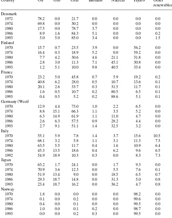
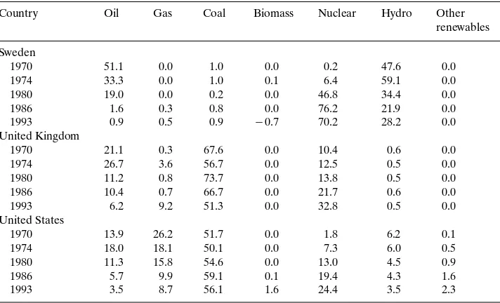
3.4. Effects of shifts in primary fuel mix for the generation of electricity and final fuel mix on aggregate carbon intensity

Examination of Tables 5 and 6 indicates the role that fuel switching for both final energy consumption and primary energy for the generation of electricity has had to contributing to the declines in aggregate carbon intensity for the residential sector. In all of the countries, there has been a pronounced shift away from the use

Ž .

of fuel oil, coal and other solid fuels in final energy consumption Table 5 . Correspondingly, there has been an increase in the consumption of both natural

Ž .

gas and electricity. Those countries Sweden, Norway and Denmark with the largest declines in aggregate carbon intensity also had the greatest reductions in the use of fuel oil. Fuel oil as a share of final energy consumption declined by over 64% in Sweden, and by nearly 45% and nearly 28% for Denmark and Norway, respectively. Since fuel oil is used for the two largest end uses, space conditioning and water heating, a shift away from this carbon-intensive fuel, particularly when replaced by lower carbon electricity in Sweden and Norway has had a significant effect on aggregate carbon intensity. Similarly, a reduction in coal as a share of final energy in the UK resulted in an almost 18% reduction in aggregate carbon intensity. Of the 10 countries, six exhibit declines in the carbon intensity of the final fuel mix, of which the majority can be explained by shifts away from fuel oil and solid fuels towards a greater use of natural gas and electricity. The rates of these shifts appear unaffected by increases or decreases in energy prices.

Table 6 provides examines the effects of shifts in the primary fuel mix used in the generation of electricity. With the exception of Italy, all of the countries exhibited declines in aggregate carbon intensity as a result of shifts in the primary fuel mix used in the generation of electricity. Those shifts were primarily away from the use of oil and coal toward a greater dependence on natural gas, and

Ž

(20)

172

.

UK with the greatest declines in aggregate carbon from this source substantially shifted power generation to nuclear power. The other four countries exhibited smaller declines, but they, too, shifted from a dependence on oil towards less carbon-intensive means of generation. These shifts seem unaffected by energy prices, and continued during periods of both high and low energy prices.

4. Conclusions

The pattern of factors leading to changes in aggregate carbon intensity from residential energy consumption in the 10 countries in this analysis vary widely across countries. Further, historical patterns of this measure for the residential sector are quite different than those for manufacturing, personal transportation, or freight end uses. For manufacturing, aggregate carbon intensity decreased by

30᎐70% over the analysis period for all countries and appears to have been driven

primarily by changes in energy price. For personal transport, aggregate carbon intensity decreased by between 1.4 and 14.5% for four of the countries, with these declines attributable to a number of factors. Aggregate carbon intensity for freight increased for all of the countries, with the exception of the UK, with increases largely correlated with growth rates in overall economic activity.

For the residential sector, changes in energy price do appear to have some effect on measures of aggregate carbon intensity, carbon emissions and energy consump-tion in some of the countries. However, changes in structure resulting from increases in per capita income have a significant role in offsetting declines resulting from increases in energy price. These offsetting shifts in structure also reduce the impacts of improvements in the energy intensity of various end uses, which result from the implementation of energy conservation measures. For the countries, where residential consumers display a sensitivity to energy prices, a 1% increase in price results in at least a 0.06% decline in carbon emissions. However, there does appear to be a threshold level of price increase required of over 2% over the analysis period for this response to occur. Examination of the index decomposition results for periods of higher energy prices does indicate that prices do have some role in promoting declines in promoting decreases in aggregate carbon intensity. Alternatively, increases in income of 1% result in between a 0.2% and 0.9% in aggregate carbon intensity as a result of shifts towards a more carbon-intensive activity mix. Without a corresponding increase in energy prices, income effects will continue to result in increases in both aggregate carbon intensity and emissions levels.

For climate mitigation policies, predicting future growth of aggregate carbon intensity from residential energy consumption then becomes an interesting issue. Increases in per capita income are expected to continue. An examination of the

Ž .

most recent period of this analysis 1985᎐1993 suggests that aggregate carbon

Ž

intensity will continue to grow from this source. For five of the countries West

.

(21)

contribution to increases in carbon intensity or offsets potential declines from shifts in other factors. These five countries also exhibit increases in carbon intensity as a result of increases in energy intensity. Not only is the activity mix becoming more carbon intensive, but also consumers are pursuing more energy

Ž

intensive energy uses e.g. an increase in the size of appliances, the choice of more energy intensive features, or an increased penetration of energy intensive end

.

uses . These types of results strongly suggest that carbon mitigation efforts, such as the implementation of energy performance standards, should be coupled with an increase in energy prices in order to be most effective. Particularly, since the ‘other’ category of energy consumption continues to grow at a much faster rate than any other end uses, and it is particularly hard to regulate the growing multitude of personal and household appliances that contribute to growth in energy consumption from this category, a pricing mechanism for carbon will undoubtedly be required to achieve carbon reduction goals.

Acknowledgements

This work was supported by the US Environmental Protection Agency, Climate Change Office and the US Department of Energy, Climate Change Research Assessment Program through the US Department of Energy under Contract Number DE-AC03-76F00098. However, financial support does not constitute an endorsement by the EPA, the DOE, Lawrence Berkeley National Laboratory, or Stratus Consulting Corporation of the views expressed in this article. The com-ments of Dr Lee Schipper, Dr Jonathan Koomey, Dr Reinhard Haas and Mary Beth Zimmerman at various points in time are gratefully acknowledged and were very helpful in crafting the final product.

Appendix A. Mathematical derivation of parametric methods 1 and 2

Carbon intensity for the residential sector is defined as carbon emissions per capita. Total residential carbon intensity may be defined as the summation over all

Ž .

end uses activities of the product of carbon emissions from the use of a final fuel type, fuel share, energy intensity for each residential end use, and activity measure per capita. That relationship is defined as follows:

m n m n

C_t C_{i jt} E_{i jt} E_{i t} A_{i t}

Ž .

Gts s

_{Ý Ý}

I a e Ri t i t jt i jts

_{Ý Ý}

1a P_t _i_s₁ _j_s₁ _i_s₁ _j_s₁ E_{i jt} E_{i t} A_{i t} P_t

Definitions of each of the variables is provided in Table A-1. For the ‘other’ category of energy consumption, the intensity and structure terms have been

Ž .

collapsed into one term Ei jtrPt to reflect the absence of comparable stock

(22)

174

Differentiating with respect to time results in:

m n m n

Dividing by Gt and integrating from 0 toT:

m n m n

A summary of notations and definitions

E_t Total energy consumption in the residential sector in yeart E_{i t} Energy consumption by activityiin yeart

Ei jt Energy consumption from the use of final energy typejby end useiin yeart

ejt Share of final energy use from final energy typejby end useiin yeart, given by,E_{i jt}rE_{i t}

Ž . At End use measure in yeart. These measures are as follows: 1 heating

Ž .

and lighting are proxied by the average floor area; 2 water heating and

Ž .

cooking are proxied by the square root of household occupancy; 3 the use of major appliances is proxied by the average number in a household

P_t Population in yeart

It Energy-activity ratio in yeartgiven byEtrAt

Ii t Energy intensity for end useiin yeartgiven byEi trAi t Ct Total carbon emissions from the residential sector in yeart Ci t Carbon emissions from end useiin yeart

Ci jt Carbon emissions from the use of final energy typejfor end useiin year

t

c_{i t} Carbon emissions share from end useiin yeart,given by,C_{i t}rC_t ci jt Carbon emissions share from the use of final energy typejfor end useiin

yeart,given by,C_{i jt}rC_t

Ri jt Rate of carbon emissions from the use of primary energy typejfor end useiin yeart, given by,C_{i jt}rE_{i jt}

Gt Aggregate carbon intensity in yeart, given by,CtrPt, or carbon emissions per capita

Ž1q%⌬Gtot 0. t Index of actual change in carbon intensity between year 0 and year t, where 0 is the first year of a period. Defined as the product of

Ž1q%⌬Gem issions 0. t, 1Ž q%⌬Gfuel 0. t, 1Ž q%⌬Gintensity 0. t, 1Ž q%⌬Gend-use 0. t,

Ž .

and 1qD0tfor a four-term index decomposition

Ž1q%⌬ Index component of estimate of the change in carbon intensity due to a

.

Gem issions 0t change in primary fuel emissions rate from the generation of electricity between year 0 and yeart

(23)

change in sectoral fuel use share between year 0 and yeart

Ž1q%⌬Gintensity 0t. Index component of estimate of the change in carbon intensity due to a change in sectoral energy intensity share between year 0 and yeart Ž1q%⌬Gen d-use 0t. Index component of estimate of the change in carbon intensity due to a

change in end-use mix between year 0 and yeart

D0t Quotient of actual carbon intensity and estimated carbon intensity, or residual of estimation

The term Ri jt essentially measures changes in the carbon intensity of electricity,

since the primary fuel mix used to generate electricity changes over time whereas

Ž .

the carbon intensity of other final fuel types e.g. natural gas are assumed to stay constant.

Both parametric methods rely on this decomposition, differing only in how they parametrize the integrals, and require the following assumptions on the paths of the components of the integrals:

4 4

where 0F␶Ft.A discrete parametrization of Eq. 3a yields the following:

m n

Simplifying and exponentiating results in an index decomposition which describes changes in total carbon intensity from residential end uses as follows:

(24)

176

The continuous parameterization requires a restatement Eq. 3a as follows:

m n m n m

The continuous parameterization then yields:

m n

(25)

m _a

Equating the discrete and continuous parametrizations results in the following weights:

Deaton, A., Muelbauer, J., 1980. Economics and Consumer Behavior. Cambridge University Press, New York.

Golove, W.H., Schipper, L.J., 1997. Restraining carbon emissions: measuring energy use and efficiency

Ž .

in the USA. Energy Policy 25 7᎐9 , 803᎐812.

Greening, L.A., Greene, D.L., 1998. Energy use, technical efficiency, and the rebound effect: a review of the literature. Experimenting with Freer Markets: Lessons From the Last 20 Years and Prospects for the Future. International Association for Energy Economics, Cleveland, OH.

Greening, L.A., Ting, M., Schipper, L., Davis, W.B., 1996. Effects of Human Behavior on Aggregate Carbon Intensity of Personal Transportation: Comparison of 10 OECD Countries for the Period 1970 to 1993, LBNL-39769. Lawrence Berkeley National Laboratory, Berkeley, CA.

(26)

178

methods: application to aggregate energy intensity for manufacturing in 10 OECD countries. Energy

Ž .

Econ. 19 3 , 375᎐390.

Greening, L.A., Davis, W.B., Schipper, L., 1998a. Decomposition of aggregate carbon intensity for the manufacturing sector: comparison of declining trends from 10 OECD countries for the period 1971

Ž .

to 1991. Energy Econ. 20 1 , 43᎐65.

Greening, L.A., McNair, M., Ottem, T., 1998b. The demand for residential energy: a factor shaping markets for innovations in technology. 19th Annual North American Conference of the United States Association for Energy Economics.

Greening, L.A., Ting, M., Davis, W.B., 1998c. Decomposition of aggregate carbon intensity for freight:

Ž .

trends from 10 OECD countries for the period 1971 to 1991. Energy Econ. in press .

Haas, R., 1997. Energy efficiency indicators in the residential sector: what do we know and what has to

Ž .

be ensured? Energy Policy 25 7᎐9 , 789᎐802.

Haas, R., Schipper, L., 1998. Residential energy demand in OECD-countries and the role of irreversible efficiency improvements. Energy Econ. 20, 421᎐442.

IEA, 1997. Indicators of Energy Use and Efficiency: Linking Energy to Human Activity. Organization for Economic Cooperation and Development International Energy Agency, Paris.

IPCC, 1995. Greenhouse Gas Inventory Reference Manual. Organization for Economic Cooperation and Development, Intergovernmental Panel on Climate Change, Paris.

Liu, X.Q., Ang, B.W., Ong, H.L., 1992. The application of the Divisia index to the decomposition of

Ž .

changes in industrial energy consumption. Energy J. 13 4 , 161᎐177.

Ž .

Lutzenhiser, L., 1992. A cultural model of household energy consumption. Energy Int. J. 17 1 , 47᎐60.

Ž .

Schipper, L., Ketoff, A.N., 1985. Residential energy use in the OECD. Energy J. 6 4 , 65᎐85. Schipper, L., Ketoff, A., Kahane, A., 1985. Explaining residential energy use by international bottom-up

comparisons. Annu. Rev. Energy 10, 341᎐405.

Schipper, L., Meyers, S., Howarth, R., Steiner, R., 1992. Energy Efficiency and Human Activity: Past Trends, Future Prospects. Cambridge University Press, Cambridge.

Schipper, L.J., Haas, R., Sheinbaum, C., 1996. Recent trends in residential energy use in OECD countries and their impact on carbon dioxide emissions: a comparative analysis of the period 1973᎐1992. Mitigat. Adapt. Strateg. Global Change 1, 167᎐196.

Schipper, L., Ting, M., Khrushch, M., Golove, W., 1998. The evolution of carbon dioxide emissions from

Ž .

energy use in industrialized countries: an end-use analysis. Energy Policy 25 7᎐9 , 651᎐672. Shinbaum, C., Schipper, L., 1993. Residential sector carbon dioxide emissions in OECD countries,

1973᎐1989: a comparative analysis. The Energy Efficiency Challenge for Europe. European Council for an Energy-Efficient Economy, Brussels.