www.elsevier.comrlocateratmos
The effects of giant cloud condensation nuclei on
the development of precipitation in convective
clouds — a numerical study
Yan Yin, Zev Levin
), Tamir G. Reisin, Shalva Tzivion
Department of Geophysics and Planetary Sciences, Raymond and BeÕerly Sackler, Faculty of Exact Sciences,Tel AÕiÕUniÕersity, P.O. Box 39040, Ramat AÕiÕ69978, Israel
Abstract
Numerical experiments are conducted to investigate the effects of giant cloud condensation
Ž .
nuclei CCN on the development of precipitation in mixed-phase convective clouds. The results show that the strongest effects of introducing giant CCN occur when the background concentra-tion of small nuclei is high, as that in continental clouds. Under these condiconcentra-tions, the coalescence between water drops is enhanced due to the inclusion of giant CCN, resulting in an early development of large drops at the lower parts of the clouds. It also leads to the formation of larger graupel particles and to more intensive radar reflectivities. When the background concentration of small nuclei is low, as in maritime clouds, the effect of the giant CCN is smaller and the development of precipitation is dominated by the droplets formed on large nuclei.q2000 Elsevier
Science B.V. All rights reserved.
Keywords: Giant CCN; Convective cloud; Numerical modeling
1. Introduction
Ž .
Cloud condensation nuclei CCN are the centers on which cloud droplets can form.
These particles range in diameter from about 0.06 mm to greater than 2mm. This wide
Ž
range of sizes has traditionally been subdivided into three classes e.g., Pruppacher and
. Ž . Ž . Ž
Klett, 1978 : small or Aitken nuclei ;0.06–0.2mm , large 0.2–2mm and giant )2
.
mm . Since small CCN are the most numerous in the atmosphere, they effectively
)Corresponding author. Fax:q972-3-6408274.
Ž .
E-mail address: [email protected] Z. Levin .
0169-8095r00r$ - see front matterq2000 Elsevier Science B.V. All rights reserved.
Ž .
determine the total concentration of droplets in a cloud. The concentrations of the small
Ž
CCN can be measured with thermal gradient diffusion cloud chambers e.g., Twomey,
.
1963; Radke and Turner, 1972; Hudson and Squires, 1976 . Although less numerous than the small CCN and much more difficult to measure, large and giant CCN provide the centers upon which larger cloud droplets can form. Under certain conditions these larger drops can lead to rapid formation of raindrop embryos.
The role of giant CCN in the initiation of warm rain had been commonly accepted for
Ž .
a long time until Woodcock et al. 1971 cast doubt on this old belief. Woodcock et al. observed the iodine–chlorine ratio of particles ranging in size from small nuclei to
raindrops sampled in Hawaii and found that the IrCl ratio in raindrops is of the same
Ž y1 2 y14 .
order as that in small nuclei 10 –10 g , but differs by one order from the ratio in
giant nuclei. They concluded that in warm oceanic tradewind clouds, giant salt nuclei
Ž .
might not be essential to the formation of raindrops. Takahashi 1976 reached similar conclusions by numerical simulation of warm rain development in a maritime cloud. In
Ž .
addition, Takahashi and Lee 1978 concluded on the basis of their improved numerical
model, that nuclei of mass less than 10y1 5g are efficient for the initiation of warm rain
and that the mass distribution of nuclei usually observed around Hawaii is the optimum distribution of nuclei for warm rain development. All of these studies are related to rain development from warm marine clouds in which the CCN concentrations are usually
less than 100 cmy3.
Ž . Ž .
Johnson 1982 investigated the role of giant and ultragiant )10 mm in radius
aerosol particles in warm rain initiation. His results showed that when ingested in growing clouds, these particles produce a tail of large drops in the cloud-droplet distribution. The effects of these large drops are more important for continental than for
Ž .
maritime clouds. Similar conclusions were also drawn by Kuba and Takeda 1983 . From the above studies one can conclude that giant CCN have little influence on the warm rain development in maritime clouds. On the other hand, the effect of such giant CCN on continental clouds could be significant. In addition, we have little knowledge about how giant CCN influence the rain formation in mixed phase clouds, especially the effects of the giant CCN on the development of the ice phase precipitation particles.
Ž .
Many measurements e.g., Eagan et al., 1974; Hindman et al., 1977; Mather, 1991 show that the precipitation development from convective clouds has been affected by the
Ž .
emission from paper mills. Mather 1991 stated that it is the addition of the ‘‘long tail’’ produced by the paper mill to the cloud-base droplet spectra that is apparently turning on, or at least enhancing, coalescence in affected storms. Numerical experiments by
Ž .
Reisin et al. 1996a showed that the precipitation from mixed convective clouds are to a larger extent, dependent on the warm microphysical processes, and that the CCN concentration and the distributions of initial droplets are the main factors determining the precipitation. It is, therefore, important to study the influences of giant CCN on the development of precipitation in cold convective clouds.
To simulate the development of precipitation particles from nuclei, the microphysical processes, especially the CCN nucleation process, needed to be treated accurately.
Ž
Different approaches have been used to deal with the CCN nucleation process e.g., Mordy, 1959; Arnason and Greenfield, 1972; Fitzgerald, 1974; Takahashi, 1976; Kuba
.
and Takeda, 1983; Flossmann et al., 1985; Kogan, 1991 . In this work, a CCN
Ž .
nucleation scheme based on Kogan 1991 has been adopted. All the microphysical
Ž
processes were solved using the multi-moments method Tzivion et al., 1987, 1989
.
Feingold et al., 1988; Reisin et al., 1996b . This method provides a solution of the kinetic transfer equations that conserves the balance between two or more physical moments in each spectral bin of the cloud particles’ distribution function.
In the following section a brief description of the numerical model is given. The initial conditions used in this study and a description of the numerical experiments is given in Section 3. The results of the numerical experiments are presented in Section 4. The discussion and conclusions follow in Section 5.
2. The cloud model
2.1. The dynamic model
The dynamic framework was a two-dimensional slab-symmetric nonhydrostatic cloud model. The wind components in the horizontal and vertical directions were calculated based on the vorticity equation and stream function. The dynamic equations were also
Ž .
solved for the virtual potential temperature perturbation uv , the specific humidity
Ž .
perturbation q , the concentration of CCN, the number and mass concentrations for
Ž .
each type of cloud particles considered For details see Appendix A .
2.2. The microphysical model
The present model was designed to simulate the evolution of precipitation particles in mixed-phase cloud starting from cloud nuclei. The warm microphysical processes included were nucleation of CCN, condensation and evaporation, collision-coalescence, and binary breakup. The ice microphysical processes included were drop freezing, ice
Ž .
nucleation deposition and condensation-freezing, and contact nucleation , ice
multipli-Ž
cation, deposition and sublimation of ice, interactions of ice–ice and ice–drop
aggrega-.
tion, accretion and riming , melting of ice particles, and sedimentation of both drops and ice particles. All the microphysical processes had been formulated using kinetic equa-tions and solved using the method of multi-moments. Three different ice species were
Ž .
considered: ice crystals, graupel particles, and snowflakes aggregates of ice crystals . Each type of particles was divided into 34 bins with mass doubling in each bin
Žxkq1s2 x , kk s1, 34 . The masses at the beginning of the first bin and the end of last.
bin for both liquid and solid phases were 0.1598=10y1 3 and 0.17468=10y3 kg,
Ž .
The temporal changes in the particles size distribution function n m, x, z, t with
Ž .
respect to mass m, at location x, z and time t, due to the microphysical processes can be generally expressed as:
dt freezing dt melting
Ž .
where n m, x, z, t is the size distribution function of the species y: water drops, icey
crystals, graupel particles, or snowflakes.
To obtain a set of moment equations for each bin for each species, the operator
Hxkq1mjd m was applied to both sides of Eq. 1. In the present study we solved for the
xk
first two moments of the category distribution function, Ny and M , the number andy
k k
mass concentrations of species y in the k th bin, respectively:
xkq1
Here y has the same meaning as above. The dependence on x, z is implicit in the above
Ž .
equations. As Tzivion et al. 1987 showed, the distribution function, n , needs to beyk
prescribed only when the integration is over an incomplete category interval. In such cases, the distribution function is approximated using a linear function, positive within the category.
The radar reflectivity factor of species y in bin k is calculated using the
nondimen-Ž .
sional parameterj that relates different moments for details see Tzivion et al., 1989 :
2 x 2 2
6 kq1 2 6 Mk
Ž .
tZyk
Ž .
t s rpH
x n x d xŽ .
sj rp ,Ž .
4N t
Ž .
xk k
and the total reflectivity factor is given by
Kmax
Z t
Ž .
sÝ Ý
ZykŽ .
t .Ž .
5ysw ,i,g ,s ks1
The radar reflectivity factor in dBZ is 10log Z with Z in mm6 my3. It should be noted
Ž .
The effective radius of hydrometers at a certain point x, z and time t was
calculated using the first two moments as:
Kmax
where, j2r3 is a nondimensional parameter that relates noninteger moments see
Ž . x
Tzivion et al. 1989 for details .
Except for the CCN nucleation process, which has been improved and will be
Ž
discussed in detail here, all the other processes were based on previous studies e.g.,
.
Tzivion et al., 1994; Reisin et al., 1996b and will only be briefly described here. We refer the interested readers to the above-mentioned papers for details.
2.2.1. Nucleation of drops
At each spatial point, the CCN of a certain size were activated when the
supersatura-tion calculated by the model exceeded the critical value determined by the Kohler
¨
Ž .
equation Pruppacher and Klett, 1997 :
A Br3
in which,n is the number of ions that results from the dissociation of a salt molecule in
Ž .
water. For NaCl, ns2, and for NH4 2SO ,4 ns3. s is the surface tension of the
solution drop. ´ is the fraction of water-soluble material of an aerosol particle. MN and
Mw are the molecular weights of CCN and water, respectively.Fs is osmotic coefficient
for the aqueous solution. rN and rw are the densities of CCN and water, respectively.
Cloud condensation nuclei begin to grow by absorption of water vapor long before they enter the cloud. These wetted particles provide the initial sizes for subsequent condensational growth. The main problem is how to include these wetted particles in the model calculations. In previous cloud models, different schemes were often adopted to
Ž .
calculate the size of these initial wet particles. Mordy 1959 assumed that at cloud base
‘‘wet’’ particles formed on nuclei smaller than 0.12 mm were at equilibrium at 100%
Ž .
relative humidity RH , and the particles formed on nuclei larger than 1.2 mm were at
Ž .
equilibrium at 99% RH. Flossmann et al. 1985 assumed that all the aerosol particles reached equilibrium with their environment at 99% RH. On the other hand, Kogan
Ž1991 assumed that the initial droplet size formed on CCN with radii smaller than 0.12.
mm were equal to the equilibrium radius at 100% RH, while for larger ones the initial
Ž .
In this study a nucleation scheme similar to Kogan 1991 was used, except that a wider size range of CCN was considered. The aerosol particles were divided into 64
Ž
categories with a minimum radius of 0.0041 mm. Based on the previous studies e.g.,
.
Mordy, 1959; Kogan, 1991 , we assumed the condensation growth of the CCN particles
with radii smaller than 0.12mm to be according to the Kohler equation. After reaching
¨
the critical sizes, these particles were then transferred to the cloud droplet bins where their subsequent growth was calculated based on the condensation equation. For the
particles with radii larger than 0.12mm, a factor k was used to calculate the initial sizes
of the droplets at zero supersaturation. The values of k and the initial radii employed in the present study are shown in Fig. 1. Factor k changes from 8.9 for the smaller CCN particles to 5 for the largest end of the CCN spectrum, to account for the smaller relative
Ž .
growth rate of the larger nuclei. The values of the factor k used by Kogan 1991 are also shown on the same plot.
2.2.2. Other microphysical processes
The immersion freezing of drops was formulated based on the measurements by Bigg
Ž1953 . According to Bigg, the number of frozen drops per unit time depends on the.
number of drops, their mass, and the supercooling. The parameterization given by
Ž .
Orville and Kopp 1977 was used in this study and the frozen drops were converted to
graupel particles, if their radii were larger than 100 mm; otherwise, they formed ice
crystals.
Nucleation of ice crystals by deposition, and condensation freezing was based on
Ž .
Meyers et al. 1992 . At each time step, the concentration of IN that could be activated was calculated according to Meyers et al. formula, and was compared with the previous number of activated ice particles. If the latter was greater than the former, no new nucleation occurred; otherwise the difference between these two values was taken as the actual number of new ice crystals that would be formed. This procedure is similar to that
Ž .
applied by Clark 1974 for nucleation of drops.
Parameterization of the number of ice crystals produced by contact nucleation due to thermophoresis, diffusiophoresis, and Brownian motion was formulated according to
Fig. 1. Initial droplet radius and the factor k used in the calculation of the CCN nucleation process as a
Ž .
Ž .
Cotton et al. 1986 . Here, ice particles formed by contact nucleation had the same mass as the drops that formed them.
The ice crystals formed by either freezing of drops smaller than 100mm in radius, or
by deposition, and condensation-freezing, were assumed to be oblate spheroids and their
initial size assumed to be 5mm in diameter. In the present paper, the shape of the ice
crystals remained unchanged with temperature, but their growth rate was allowed to vary w
with temperature as if the ice particles changed their shape for details see Reisin et al.
Ž1996b ..x
The changes in the mass and number distribution functions of the drops and the ice
particles due to diffusive growthrevaporation of water vapor, were calculated for each
Ž .
size category by analytically solving for one time step the kinetic diffusion equation
ŽTzivion et al., 1989; Reisin et al., 1992,1996b ..
The model considered collision coagulation between the different species, as well as
w Ž . x
collision breakup of drops Low and List 1982a,b kernels . Such interactions could lead to the transformation from one particle type to another. In this study we made the following assumptions:
1. Snow particles were formed and grew by aggregation of ice crystals.
2. Ice crystals grew by riming with drops smaller than themselves, as long as the overall rimed mass was less than the mass of the ice crystal itself; otherwise the ice crystal was transformed into a graupel particle.
3. The interactions between graupel and other particles always produced graupel. 4. Graupel particles were also created when drops collided with snow particles and with
ice crystals smaller than themselves.
The collision and coalescence efficiencies used for interactions between drop–drop,
Ž .
drop–ice, and ice–ice were similar to those in Reisin et al. 1996b . For collision
Ž .
between drops, the kernel of Low and List 1982a,b are used for raindrops larger than
Ž .
0.6 mm; the coalescence efficiencies of Ochs et al. 1986 are employed as collection
Ž .
efficiencies assuming that the collision efficiencies in this region are close to unity in
Ž .
the region 0.1–0.6 mm; the collision efficiencies of Long 1974 are adapted for smaller drops. The collision efficiencies between graupel particles and drops are calculated
Ž . Ž .
according to Hall 1980 and Rasmussen and Heymsfield 1985 . For ice crystals
Žplates colliding with drops we used collision efficiencies given by Martin et al. 1982. Ž .
and for large supercooled drops colliding with planar ice crystals we used the
coeffi-Ž .
cients calculated by Lew et al. 1985 . The data sets for ice and drop as collectors were combined to give a full set of size ranges. But, there is not enough information to cover
Ž .
the whole size range required by the model. An approach suggested by Chen 1992 was used to fill the gaps in the data. This approach was based on the fact that the collision efficiency reaches a minimum when the drop being collected reaches a size such that its fall velocity approaches that of the collector ice particle, and that for drops of even larger sizes, the relative velocity between drop and ice crystal changes sign and the collision efficiency increases again. A mirror image about the minimum of the collision efficiencies was assumed so that interpolations could be made between existing data. For
Ž .
efficiencies remain virtually unchanged and have been assumed to be constant for a fixed ice crystal size. Coalescence efficiencies for interaction between ice particles are
Ž .
used in accordance with Wang and Chang 1993 , in which the dependence on
temperature was considered.
The Hallett–Mossop mechanism for secondary ice production was parameterized
Ž .
according to Mossop 1978 , in which the number of ice crystals produced per second
Ž .
was formulated as a function of the number of large drops G24.8mm and small drops
ŽF12.3mm collected per second by a graupel particle. The temperature dependence of.
Ž .
this process was taken from Cotton et al. 1986 , where the maximum occurs at
;y58C.
The kinetic equation for the melting of graupel particles was treated in the same way as the evaporation, except that the rate of change of mass of a melting graupel depended
Ž .
on temperature Rasmussen and Heymsfield, 1987 . We assumed complete shedding of the melted mass for the graupel particles. Snowflakes and ice crystals were assumed to melt instantaneously whenever they entered a region in which the environmental
temperature was above 08C.
Sedimentation of both drops and ice particles was calculated using Smolarkiewicz
Ž1983 positive advection scheme. The parameters for terminal fall velocity of drops.
Ž . Ž .
were according to Beard 1977 and for the ice particles based on Bohm 1989 .
¨
The grid dimensions of the model were set to 300 m both in the horizontal and the
Ž
vertical directions separate experiments indicated that the simulation results were not
.
sensitive to the changes in the grid size . The vertical and the horizontal dimensions of the domain were 12 and 30 km, respectively. The time step was 5 s for dynamic and the
Ž .
microphysical processes except for the diffusive growthrevaporation or sublimation
processes of hydrometeors, in which a time step of 2.5 s was used.
3. Description of the experiments and initial conditions
The initial total aerosol spectrum was based on the measurements carried out in
Ž .
Montana, USA, by Hobbs et al. 1985 . We fitted this spectrum by superimposing three lognormal distributions as:
The parameters of the distributions were similar to those used by Respondek et al.
Table 1
Parameters for the aerosol particle distribution: nistotal number of aerosol particles per cubic centimeter of air, Risgeometric mean aerosol particle radius inmm, sisstandard deviation in mode i
Mode i ni Ri logsi
1 40 000 0.006 0.3
2 3980 0.03 0.3
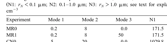
Table 2
Percentages of water soluble particles in modes 1, 2 and 3, and the CCN concentrations in the three classes
ŽN1: rN-0.1mm; N2: 0.1–1.0mm; N3: rN)1.0mm; see text for explanations . The concentration is in.
cmy3
Experiment Mode 1 Mode 2 Mode 3 N1 N2 N3
MR0 0.2 8 0.0 171.5 5.30 0.0
MR1 0.2 8 50 171.5 5.34 0.02
CN0 5 20 0.0 1029.8 13.25 0.0
CN1 5 20 50 1029.8 13.30 0.02
EC0 10 20 0.0 1697.6 13.27 0.0
EC1 10 20 50 1697.6 13.31 0.02
EC2 10 20 100 1697.6 13.36 0.05
Ž1995 and are given in Table 1. The concentration was assumed to decrease with height.
according to:
N z , r
Ž
n.
sN zŽ
s0, rn.
=expŽ
yzrzs.
,Ž .
10where, z was the scale height and set to 2 km in this study.s
As mentioned above, because the main objective here was to study the effects of size distributions of CCN on the development of mixed convective clouds, the variations of the chemical compositions of the aerosol particles were not considered. Instead, the CCN spectra were created by simply assuming different percentages of total aerosol particles to be water-soluble. In addition, all the CCN particles were assumed to be composed of ammonium sulfate. This assumption was also based on the previous studies
Že.g., Fitzgerald, 1974; Takeda and Kuba, 1982 which showed that the differences in.
Ž Ž . .
the chemical composition of CCN such as NaCl, and NH4 2SO4 do not significantly
change the predicted size distribution of cloud droplets. The fractions of water soluble
Ž .
particles ´ in Eq. 8 multiplied by 100 and the CCN number for each class are shown
in Table 2 and all the initial CCN distributions are given in Fig. 2. The experiments
Ž . Ž .
were divided into three groups, ‘maritime’ MR , ‘continental’ CN , or
‘extreme-con-Ž .
tinental’ EC , based on their CCN concentrations. In each group at least two cases were
Ž .
studied. In the first set of experiments, MR0, CN0 or EC0 hereafter, control cases , the initial CCN were assumed to contain particles only from the first two modes of aerosol
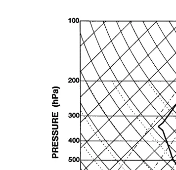
Fig. 3. Vertical profiles of temperature and dew point used in the present work.
distributions, while the third mode was assumed to be water insoluble. In the second set, MR1, CN1 or EC1, the concentration of the Aitken and large particles were left as
Ž y1 .
before but a third mode was added, which contained 50% soluble particles ;23 l .
Ž .
In the extreme-continental group, a third case EC2 with twice the concentration of giant CCN was also tested.
The initial thermodynamic conditions for all reported tests here were given by a theoretical profile of temperature and dew point as shown in Fig. 3. The temperature,
dew point temperature, and pressure at the surface were 268C, 15.88C, and 1007 hPa,
respectively. For initialization, a pulse of heat that produced a 28C perturbation was
applied for one time step at ts0 at a height of 600 m, and at the center of the domain.
The possible influence of wind shear was not considered in the present study.
4. Results
Ž
Numerical simulations were carried out until the cloud dissipated usually 60 min
. Ž .
from model initiation . In all the cases the cloud base and top were at 1.5 km 118C and
Ž .
7.2 km y288C , respectively. The 08C isotherm was at 2.7 km. The base and the top of
the cloud were defined as the place where the total mixing ratio of the hydrometeors was
y1Ž .
greater than 0.01 g kg as Orville and Kopp, 1977 . The rain initiation was defined as
the time at which the maximum rainfall rate at the surface began to exceed 0.1 mm hy1.
A summary of the main results obtained for seven runs is presented in Table 3. Below, we compare the cases for each group.
( )
4.1. Continental clouds CN
Ž .
Two cases CN0 and CN1 were calculated for continental clouds. The general appearance of these two clouds in the developing stage was similar. The clouds began to form 15 min after the model initialization, and continued to develop very rapidly after
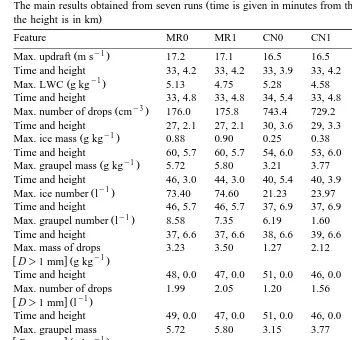
Table 3
Ž
The main results obtained from seven runs time is given in minutes from the initiation of the calculations and
.
the height is in km
Feature MR0 MR1 CN0 CN1 EC0 EC1 EC2
y1
Ž .
Max. updraft m s 17.2 17.1 16.5 16.5 16.3 16.3 16.2
Time and height 33, 4.2 33, 4.2 33, 3.9 33, 4.2 33, 3.9 33, 3.9 33, 3.9
Max. number of drops cm 176.0 175.8 743.4 729.2 1134 1102 1080
Time and height 27, 2.1 27, 2.1 30, 3.6 29, 3.3 30, 3.6 30, 3.6 30, 3.3
Max. graupel mass g kg 5.72 5.80 3.21 3.77 2.58 3.63 3.99
Time and height 46, 3.0 44, 3.0 40, 5.4 40, 3.9 41, 5.1 40, 3.9 39, 4.5
y1
Ž .
Max. ice number l 73.40 74.60 21.23 23.97 20.63 22.90 23.50
Time and height 46, 5.7 46, 5.7 37, 6.9 37, 6.9 37, 6.9 37, 6.9 37, 6.9
y1
Ž .
Max. graupel number l 8.58 7.35 6.19 1.60 3.98 0.63 0.68
Time and height 37, 6.6 37, 6.6 38, 6.6 39, 6.6 40, 6.3 39, 6.6 37, 6.3
Max. mass of drops 3.23 3.50 1.27 2.12 0.45 1.86 2.12
y1 wD)1 mm g kgxŽ .
Time and height 48, 0.0 47, 0.0 51, 0.0 46, 0.0 49, 0.0 45, 0.0 44, 0.0
Max. number of drops 1.99 2.05 1.20 1.56 0.54 1.46 1.63
y1 wD)1 mm lxŽ .
Time and height 49, 0.0 47, 0.0 51, 0.0 46, 0.0 49, 0.0 46, 0.0 45, 0.0
Max. graupel mass 5.72 5.80 3.15 3.77 2.53 3.63 3.99
y1 wD)1 mm g kgxŽ .
Time and height 46, 3.0 44, 3.0 40, 5.4 40, 3.9 41, 5.1 40, 3.9 39, 4.5
Max. graupel number 1.05 0.92 1.10 0.32 0.82 0.28 0.35
y1 wD)1 mm lxŽ .
Time and height 36, 6.0 36, 5.7 39, 6.0 37, 6.0 41, 5.7 37, 6.0 37, 6.0
Time of rain initiation 38 36 41 36 42 36 35
Ž .
Max. radar reflectivity dBZ 67.6 68.0 59.9 64.4 55.5 63.4 64.0
Time and height 46, 3.6 46, 3.3 45, 3.3 41, 3.0 42, 4.2 39, 4.5 39, 4.2
y1
Ž .
Max. rain rate mm h 187.0 196.9 59.0 101.5 21.3 86.1 100.1
Time 49 48 51 46 50 45 45
Ž .
Max. accumulated rain mm 27.25 29.18 7.76 12.45 2.57 10.27 12.05
thermodynamic conditions and to a lesser extent to the more latent heat released by
Ž
formation of ice phase hydrometeors ice nucleation by deposition and
condensation-.
freezing started at temperatures lower thany58C . The clouds reached their maximum
Ž .
development 33 min from model initialization Table 3 and the maximum updraft was 16.5 m sy1.
Although the dynamic structure was similar, many of the microphysical properties
Ž .
were different Table 3 . Fig. 4 shows the mass and number distribution functions of the
Ž .
drops at the cloud center, at 1800 m height just above cloud base , and after 16 min of
Ž . Ž .
simulation corresponding to the stage of cloud initiation in CN0 heavy line and CN1
Žthin line . It is obvious from this figure that although their numbers were relatively.
Ž . Ž . Ž . Ž
Fig. 4. Mass left and number right distribution functions of drops for case CN0 heavy line and CN1 thin
. Ž .
line at the center of the clouds, 1800 m high just above the cloud base , and at 16 min of simulation.
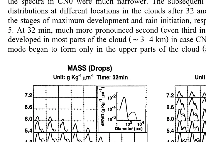
the spectra in CN0 were much narrower. The subsequent evolution of the drop size
Ž
distributions at different locations in the clouds after 32 and 36 min corresponding to
.
the stages of maximum development and rain initiation, respectively are shown in Fig.
Ž .
5. At 32 min, much more pronounced second even third in some of the points modes
Ž .
developed in most parts of the cloud ;3–4 km in case CN1, while in CN0 the second
Ž .
mode began to form only in the upper parts of the cloud above 4 km . These results
Ž . Ž .
Fig. 5. Mass distribution functions of drops in case CN0 heavy line and CN1 thin line at different spatial
Ž . Ž .
demonstrate that the coalescence process in CN1 began to operate earlier and more efficiently than that in CN0. Because larger drops developed earlier in CN1, they descended to the lower reaches of the cloud after 36 min. In contrast, in CN0 at the same time, most of the large drops were still growing in the middle and upper parts of the cloud.
Consistent with the development of the drop size distributions, the cloud in CN1 reached its maximum LWC, 1 min earlier and 600 m lower than that in CN0, but the values of maximum LWC and drop number were smaller in CN1 than in CN0. These results show that the inclusion of giant CCN in CN1 inhibited the nucleation of some of the smaller CCN and accelerated the growth of precipitation by transferring more liquid
Ž .
water to millimeter size raindrops Table 3 .
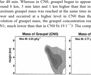
Comparison of the graupel production between case CN0 and CN1 is given in Fig. 6. In CN1, graupel particles initially formed at 32 min of simulation near the 5 km
Ž;y158C level reached their maximum mass of 3.77 g kg. y1 at the height of 3.9 km
after 40 min. Whereas in CN0, graupel began to appear after 35 min and at the height around 6 km, 3 min later and 1 km higher than that in the former case. Although the maximum graupel mass was reached at the same time in these two cases, the value was lower and occurred at a higher level in CN0 than that in CN1. Different from the
evolution of graupel mass, the graupel concentration reached a peak of only 1.6 ly1 in
Ž y1.
CN1, much lower than that in CN0 6.19 l . The comparatively larger mass and lower
Ž . Ž .
Fig. 6. Time–height cross sections of mass upper and concentration lower of graupel particles for case CN0
Žleft and CN1 right . The unit used and maximum value obtained are shown at the upper left corner of each. Ž .
Ž .
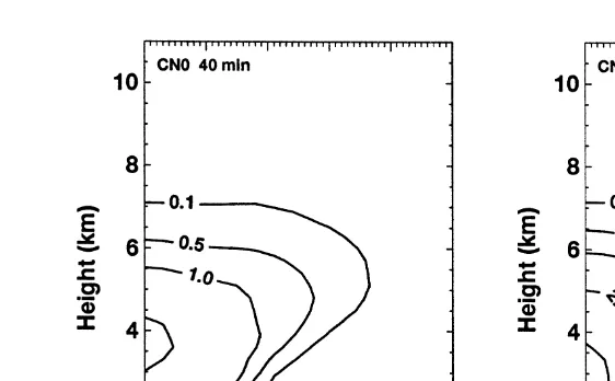
Fig. 7. Spatial distribution of the effective radii of graupel particles at 40 min in case CN0 left and CN1
Žright . Unit: mm..
concentration of graupel in CN1 correspond to larger sizes than those in CN0, as can be seen in Fig. 7.
Fig. 7 shows the spatial distribution of the effective radii of graupel particles at 40
Ž .
min corresponding to the maximum development of graupel content . It can be seen
Ž .
that larger graupel particles reff)2 mm appeared in the lower part of the cloud in case
CN1, while they were almost absent in CN0. In addition, the figure shows that some of the large graupel particles had already fallen to the ground in CN1. In CN0, on the other hand, all the particles were still being lifted in the middle and upper parts of the cloud.
Ž .
Because of their relatively small sizes, the particles reff-0.5 mm in CN0 were also
carried farther away from the main updraft core.
The difference in the content and concentration of ice crystals between CN0 and CN1 can be found in Table 3. Compared with CN0, more ice crystals were produced in CN1.
Ž .
Fig. 8. Time–height cross sections of the radar reflectivity at cloud center for cases CN0 left and CN1
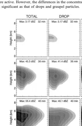
This is due to the higher supersaturation with respect to ice in CN1, which enhanced the formation of ice crystals by deposition and condensation-freezing, and the relatively large graupel particles and drops, which made the secondary ice production process more active. However, the differences in the concentration and mass of ice crystals were not significant as that of drops and graupel particles.
Ž . Ž .
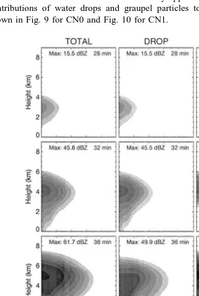
Fig. 9. The total radar reflectivity left , the contribution of water drops middle , and the contribution of
Ž . Ž
The time–height cross sections of the radar reflectivity in cases CN0 and CN1 are
presented in Fig. 8. They10 dBZ echo developed about 5 min earlier in CN1 than that
in CN0, and the maximum echo reached about 5 dBZ higher in the former. It is also noted that in CN1 the initial radar reflectivity appeared at a lower height. The relative contributions of water drops and graupel particles to the total radar reflectivity are shown in Fig. 9 for CN0 and Fig. 10 for CN1.
Ž . Ž .
Fig. 10. The total radar reflectivity left , the contribution of water drops middle , and the contribution of
Ž .
Ž
In case CN0, the first echo appeared at 32 min from model initiation 16 min after
.
cloud formation and was mainly produced by graupel particles. Only at the very beginning stage, the contribution from supercooled water was more than that from graupel. In case CN1, however, the initial echo appeared at 26 min of simulation due to the early growth of the large drops. Although the echo from the graupel particles became very strong about 10 min later, the total contribution to the radar reflectivity was nearly equally shared by both types of hydrometeors.
Consistent with the development of precipitation particles, rain in case CN1 started 5 min earlier, reached a higher intensity, and produced more rain on the ground than that in CN0.
( )
4.2. Maritime clouds MR
Ž .
Two simulations MR0 and MR1 were performed for the maritime clouds. Here, one must keep in mind that the term ‘maritime cloud’ in this study only refers to the relatively small initial CCN concentration.
The clouds simulated in these two cases had the same dynamic structure, in terms of
Ž .
maximum updrafts and the time and altitude of these maximums Table 3 . Both clouds reached their peak liquid water content after 33 min of simulation at a height of 4.8 km.
The maximum mass in case MR0 and MR1 was 5.13 and 4.75 g kgy1, respectively.
Although the inclusion of giant CCN slightly reduced the liquid water content, the maximum drop concentration was almost the same in these two cases. This fact can be explained by the evolution of the drop size distribution. Figs. 11 and 12 show the drop size distribution of case MR0 and MR1 at 16 and 36 min, respectively. Comparing these
Ž .
figures with the corresponding ones in continental clouds Figs. 4 and 5 reveals that
Ž
when the CCN concentration in the Aitken and large size mode were low maritime
.
clouds — although inclusion of giant CCN produces a few large drops at the initial
Ž .
stage 16 min of the cloud — the droplets formed on large CCN caught up with them
Ž
due to their rapid growth under the higher supersaturation compared to the continental
.
clouds produced in the updraft region. In addition, because the drops formed on the
Ž . Ž . Ž .
Fig. 11. Mass left and number right distribution functions of drops for case MR0 heavy line and MR1
Ž . Ž .
Fig. 12. Mass distribution functions of drops in case MR0 heavy line and MR1 thin line at different spatial points, and at 36 min of simulations.
large CCN were more numerous than those formed on giant CCN, they dominated the subsequent collection of drops, and reduced the relative advantage of the latter. This fact can also be seen from the similar development of the graupel particles in Table 3.
In both cases, the graupel particles began to form at 31 min, and 6 min later the peak concentration appeared at 6.6 km. The maximum graupel number in case MR0 and MR1
were 8.58 and 7.35 ly1, and maximum masses were 5.72 and 5.80 g kgy1, respectively.
Ž .
The peak values were located at the same altitude Table 3 . Due to the similarity of the
Ž
development of the precipitation particles, the evolution of the radar reflectivity not
. Ž
shown was also very similar maximum radar reflectivity in case MR0 and MR1 were
.
67.6 and 68 dBZ, respectively . A small difference in the height of the maritime echo appeared in MR1 that occurred about 0.3 km lower. Table 3 shows that the time of rain initiation, rainfall rate and accumulated rain were similar in MR0 and MR1. In summary, the effects of introducing giant CCN to maritime clouds were relatively small.
( )
4.3. Extreme-continental clouds EC
Ž .
Three simulations EC0, EC1 and EC2 were conducted for the extreme-continental
Ž .
clouds in order to investigate i how the giant CCN influence the development of
Ž .
Although different number of giant CCN were included in the initial CCN spectra, the developments of the cloud dynamic structures in these three cases were almost the same and also very similar to the continental cases described before. The clouds reached their maximum development at 33 min of simulation and the peak updraft was 16.3 m
sy1, located at 3.9 km high. As expected, more significant differences, compared with
the continental cases, appeared in the development of the hydrometers between the control case and the case with giant CCN.
4.3.1. Comparison between case EC0 and EC1
The time–height cross sections of drops and graupel particles at the clouds center are shown in Figs. 13 and 14. Although in both cases, cloud began to form at the same time the cloud reached its maximum LWC earlier and located at a lower altitude in EC1 than in EC0, and maximum value was smaller in the former case than in the latter. The maximum drop number in case EC1 was also slightly lower than that in EC0.
The most striking differences are exhibited in the development of graupel particles. The inclusion of giant CCN in EC1 accelerated the growth of drops by collision-coales-cence mechanism. At the same time, this also reduced the overall concentration of the drops. Therefore, when the drops were lifted above zero degree level, the concentration
Ž . Ž .
Fig. 13. Time–height cross sections of liquid water content upper and drop number lower at cloud center
Ž . Ž .
Ž . Ž .
Fig. 14. Time–height cross sections of graupel content upper and number lower at cloud center for case
Ž . Ž .
EC0 left and EC1 right . The unit used and maximum value obtained are shown at the upper left corner of each panel.
of graupel particles formed by self-freezing and interactions between drops and ice particles was lower in EC1 than in EC0. This is manifested in the results shown in Table 3, that is, the concentration of graupel particles in EC1 only reached a maximum of 0.63
ly1, much lower than that in EC0, 4 ly1. On the other hand, the graupel mass in EC1
reached a maximum of 3.63 g kgy1, higher than in EC0, 2.58 g kgy1. The location of
peak value was also 1.2 km lower in EC1 than in EC0.
Comparison of the radar reflectivity between case EC0 and EC1 is presented in Fig. 15. Consistent with the development of precipitation particles the radar reflectivity in case EC1 grew faster and reached a higher peak echo than in case EC0. The difference of radar reflectivity between EC1 and EC0 was 8 dBZ, again larger than in the continental cases, 4.5 dBZ, and in maritime cases, 0.4 dBZ.
These results indicate that the differences in precipitation particles produced by inclusion of giant CCN in extreme-continental clouds are more significant than that in the moderate continental clouds. This is also expressed in the earlier initiation of rain
Žalmost 6 min in EC1 see Table 3 , and the higher rain intensity. The maximum rain. Ž .
Ž .
intensity increased by a factor of three due to the inclusion of giant CCN case EC1 , the
Ž .
Ž .
Fig. 15. Time–height cross sections of the radar reflectivity at cloud center for cases EC0 left and EC1
Žright ..
4.3.2. Comparison between case EC2 and EC1
In EC2 the concentration of giant CCN in the reference case EC0 was doubled. The main results obtained from this simulation are listed in Table 3. It can be seen that the dynamic fields such as updraft and LWC in case EC2 were very similar to EC1, but the differences between EC2 and EC0 were more pronounced than that between EC1 and EC0. Both the content and concentrations of raindrops and graupel particles were increased with increasing concentration of giant CCN. The results in Table 3 also show that with increased concentration of giant CCN, the rain started earlier, reached higher intensity and produced more total rain on the ground. Correspondingly, the radar reflectivity also reached higher values. One should also note, however, that although increase in the concentration of giant CCN results in more precipitation at the surface, too many giant CCN could lead to stronger competition among the droplets formed on them, leading to reduction of precipitation.
5. Discussion and conclusions
The principal conclusions of this study are that inclusion of giant CCN produces a tail of large drops in the cloud droplet distribution near cloud base. The effects of these large drops are significant when the concentration of small nuclei is high, as that in continental or especially, in extreme-continental clouds. Under these conditions, the inclusion of giant CCN accelerates coalescence between water drops, leading to an early development of large drops at the lower parts of the clouds. It also leads to the formation of larger graupel particles and more intensive radar reflectivity. When the concentration of small nuclei is low, as that in maritime clouds, the effect of the giant CCN is small and the development of precipitation is dominated by the droplets formed on large nuclei. We will elaborate these points further below.
Inclusion of giant CCN always produces a few large droplets at the cloud initiation
Ž .
CCN is high, the droplets grow slow because of their higher concentrations and the increased competition for the available supersaturation produced by the updrafts. As a result, raindrops cannot be formed effectively by the collision and coalescence process and the cloud exists in a colloidal stable state. In this case, the large droplets formed on giant CCN serve as an inherent destabilizing factor, which accelerates the collision and coalescence between drops in the lower parts of the clouds. This is seen in the drop size distributions and radar reflectivity in Section 4.1. In contrast, in maritime clouds in which the concentration of smaller CCN is low, the droplets formed on large CCN grow rapidly due to the low concentration of total droplets and the reduced competition for the available water vapor. Because they are more numerous than the drops formed on giant CCN, these drops dominate the subsequent collection process. This means that the relative advantage or ‘‘Head start’’ of the drops formed on the giant CCN is reduced. The role of the giant CCN is not only in the development of larger drops but also in the acceleration of precipitation development through the ice phase. As was shown here, precipitation is produced in the extreme-continental cloud even without the presence of giant CCN. This is due to the formation of ice by nucleation. But the important conclusion here is that the initiation time, the location, and the quantity of these precipitation particles is very much different when even a few giant CCN are presented. This can be attributed to the fact that both the freezing and accretion processes are dependent on the drop sizes under the same thermodynamic conditions. The relatively large drops formed in the case with giant CCN produce graupel particles earlier. Because of their higher coagulation efficiency with drops, these early appearing graupel particles capture more droplets and grow faster as they are lifted in the updraft region. In addition, because of their larger size, these graupel particles are not lifted to higher altitudes and remain closer to cloud base. In contrast, in the control case, the more numerous but smaller drops are transported to the upper parts of the cloud where they grow or form ice particles by freezing or through interaction with ice particles. Since these particles are smaller in size, they are also carried farther away from the updraft core by the divergent flow that exists in the upper reaches of the cloud.
When large drops are carried into the supercooled regions, ice multiplication pro-cesses may also takes effect under suitable temperature conditions. As has been indicated in the previous section, inclusion of giant CCN leads to the formation of large drops and graupel particles that develop earlier and at lower levels in the clouds, and this in turn increases the opportunities for ice multiplication. This may explain the reason why more ice crystals are produced in the cases when giant CCN are included.
The results presented in this paper are based on a specific thermodynamic profile,
Ž .
which represents a moderate convective cloud with relatively warm cloud base 118C .
Although the principal effects of the giant CCN on cloud and precipitation development are not expected to be much different under different atmospheric conditions, more numerical experiments are needed to draw a firm conclusion.
Acknowledgements
contribution to the laboratory, which made part of this work possible. Comments by Professor K.D. Beheng helped us clarify some important points and improved the quality of this paper. We thank him for that. Part of the calculations was carried out using the Cray J932 computer of Inter University Computer Center, Israel.
Appendix A. Dynamic equations of the model
The vertical and horizontal velocity were calculated based on the stream function and vorticity equation as follows:
then u and w components of the wind speed can be calculated by
1 Ec 1 Ec
us ,ws y
Ž
A3.
r0 Ez r0 Ex
c is the stream function, uÕ the virtual potential temperature deviation from the
Ž .
environmental virtual potential temperatureuÕ, and My ysw, i, g, s are the specific
0
Ž
liquid and solid water contents ‘i’ for ice crystals, ‘g’ for graupel particles, and ‘s’ for
.
snow particles .
The prediction equations for the virtual potential temperature perturbation uÕ, the
specific vapor perturbation q, the concentration and mass of a specific bin for water
drops and ice particles, Nwk and Mwk and the CCN size distribution function nCCNk were
Ž .
similar to those in Reisin et al. 1996b , except that the definitions of advective and
Ž . Ž .
turbulent diffusion operators, D f and Fd, q f , were different in the present model
and can be expressed as:
f being an arbitrary function;nd, q is the turbulent coefficient based on the approach of
Ž .
Monin and Yaglom 1968 :
2 2 2 0 .5
< <
where
The value of C was chosen to make the simulations stable as was done in Reisin ett
Ž .
al. 1996b .
References
Arnason, G., Greenfield, R., 1972. Micro- and macro-structure of numerically simulated convective clouds. J. Atmos. Sci. 29, 342–367.
Beard, K.V., 1977. Terminal velocity adjustment for cloud and precipitation. J. Atmos. Sci. 34, 1293–1298. Bigg, E.K., 1953. The formation of atmospheric ice crystals by the freezing of droplets. Q. J. R. Meteorol.
Soc. 79, 510–519.
Bohm, H.P., 1989. A general equation for the terminal fall speed of solid hydrometeors. J. Atmos. Sci. 46,¨ 2419–2427.
Chen, J.P., 1992. Numerical simulation of the redistribution of atmospheric trace chemicals through cloud processes. PhD Thesis. The Pennsylvania State Univ., University Park, PA 16802, 342 pp.
Clark, T.L., 1974. On modeling nucleation and condensation theory in Eulerian spatial domain. J. Atmos. Sci. 31, 2099–2117.
Cotton, W.R., Tripoli, G.J., Rauber, R.M., Mulvihill, E.A., 1986. Numerical simulations of the effects of varying ice crystal nucleation rates and aggregation processes on orographic snowfall. J. Clim. Appl. Meteorol. 25, 1658–1680.
Eagan, R.C., Hobbs, P.V., Radke, L.F., 1974. Particle emissions for a large Kraft paper mill and their effects on the microstructure of warm clouds. J. Appl. Meteorol. 13, 535–552.
Feingold, G., Tzivion, S., Levin, Z., 1988. The evolution of raindrop spectra: Part I. Stochastic collection and breakup. J. Atmos. Sci. 45, 3387–3399.
Fitzgerald, J.W., 1974. Effect of aerosol composition on cloud droplet size distribution: a numerical study. J. Atmos. Sci. 31, 1358–1367.
Flossmann, A.I., Hall, W.D., Pruppacher, H.R., 1985. A theoretical study of the wet removal of atmospheric pollutants: Part I. The redistribution of aerosol particles captured through nucleation and impaction scavenging by growing cloud drops. J. Atmos. Sci. 42, 582–606.
Hall, W.D., 1980. A detailed microphysical model within a two-dimensional dynamic framework: model description and preliminary results. J. Atmos. Sci. 37, 2486–2507.
Hindman, E.E. II, Hobbs, P.V., Radke, L.F., 1977. Cloud condensation nuclei from a paper mill: Part I. Measured effect on clouds. J. Appl. Meteorol. 16, 745–752.
Hobbs, P.V., Bowdle, D.A., Radke, L.F., 1985. Particles in the lower troposphere over the high plains of the United States: Part I. Size distributions, elemental composition and morphologies. J. Clim. Appl. Meteorol. 24, 1344–1356.
Hudson, J.G., Squires, P., 1976. An improved continuous flow diffusion cloud chamber. J. Appl. Meteorol. 15, 776–782.
Johnson, D.B., 1982. The role of giant and ultragiant aerosol particles in warm rain initiation. J. Atmos. Sci. 39, 448–460.
Kogan, Y.L., 1991. The simulation of a convective cloud in a 3-D model with explicit microphysics: Part I. Model description and sensitivity experiments. J. Atmos. Sci. 48, 1160–1189.
Lew, J.K., Kingsmill, D.E., Montague, D.C., 1985. A theoretical study of the collision efficiency of small planar ice crystals colliding with large supercooled water drops. J. Atmos. Sci. 42, 857–862.
Long, A.B., 1974. Solutions to the droplet coalescence equation for polynomial kernels. J. Atmos. Sci. 11, 1040–1057.
Low, T.B., List, R., 1982a. Collision coalescence and breakup of raindrops: Part I. Experimentally established coalescence efficiencies and fragments size distribution in breakup. J. Atmos. Sci. 39, 1591–1606. Low, T.B., List, R., 1982b. Collision coalescence and breakup of raindrops: Part II. Parameterization of
fragment size distributions in breakup. J. Atmos. Sci. 39, 1607–1618.
Martin, J.J., Wang, P.K., Pruppacher, H.R., 1982. A numerical study of the effect of electric charges on the efficiency with which planar ice crystals collect supercooled cloud drops. J. Atmos. Sci. 38, 2462–2469. Mather, G.K., 1991. Coalescence enhancement in large multicell storms caused by the emissions from a Kraft
paper mill. J. Appl. Meteorol. 30, 1134–1146.
Meyers, M.P., DeMott, P.J., Cotton, W.R., 1992. New primary ice-nucleation parameterizations in an explicit cloud model. J. Appl. Meteorol. 31, 708–721.
Monin, A.C., Yaglom, A.M., 1968. In: Statistical Hydromechanics. Izdatel’stvo Nauka, p. 2.
Mordy, W., 1959. Computation of the growth by condensation of a population of cloud droplets. Tellus 11, 16–44.
Mossop, S.C., 1978. The influence of drop size distribution on the production of secondary ice particles during graupel growth. Q. J. R. Meteorol. Soc. 104, 323–330.
Ochs, H.T., Czys, R.R., Beard, K.V., 1986. Laboratory measurements of coalescence efficiencies for small precipitating drops. J. Atmos. Sci. 43, 225–232.
Orvile, H.D., Kopp, F.J., 1977. Numerical simulation of the life history of a hailstorm. J. Atmos. Sci. 34, 1596–1618.
Pruppacher, H.R., Klett, J.D., 1997. Microphysics of Clouds and Precipitation. Reidel, 954 pp.
Radke, L.F., Turner, F.M., 1972. An improved automatic cloud condensation nucleus counter. J. Appl. Meteorol. 11, 105–109.
Rasmussen, R.M., Heymsfield, A.J., 1985. A generalized form for impact velocities used to determine graupel accretional densities. J. Atmos. Sci. 42, 2275–2279.
Rasmussen, R.M., Heymsfield, A.J., 1987. Melting and shedding of graupel and hail: Part I. Model physics. J. Atmos. Sci. 44, 2754–2763.
Reisin, T., Levin, Z., Tzivion, S., 1996a. Rain production in convective clouds as simulated in an axisymmet-ric model with detailed microphysics: Part II. Effects of varying drops and ice initiation. J. Atmos. Sci. 53, 1815–1837.
Reisin, T., Levin, Z., Tzivion, S., 1996b. Rain production in convective clouds as simulated in an axisymmetric model with detailed microphysics: Part I. Description of the model. J. Atmos. Sci. 53, 497–519.
Reisin, T., Tzivion, S., Levin, Z., 1992. The influence of warm microphysical processes on ice formation and diffusional growth — a numerical study. In: 11th Int. Conf. Clouds Precip., Montreal, Canada, 17–21 August. pp. 280–283.
Respondek, P.S., Flossmann, A.I., Alheit, R.R., Pruppacher, H.R., 1995. A theoretical study of the wet
Ž .
removal of atmospheric pollutants: Part V. The uptake, redistribution, and deposition of NH4 2SO by a4 convective cloud containing ice. J. Atmos. Sci. 52, 2121–2132.
Smolarkiewicz, P.K., 1983. A simple positive definite advection scheme with small implicit diffusion. Mon. Weather Rev. 111, 479–486.
Takahashi, T., 1976. Warm rain, giant nuclei and chemical balance — a numerical model. J. Atmos. Sci. 33, 269–286.
Takahashi, T., Lee, S., 1978. The nuclei mass range most efficient for the initiation of warm cloud showers. J. Atmos. Sci. 35, 1934–1946.
Takeda, T., Kuba, N., 1982. Numerical study of the effect of CCN on the size distribution of cloud droplets: Part I. Cloud droplets in the stage of condensation growth. J. Meteorol. Soc. Jpn. 60, 978–993. Twomey, S., 1963. Measurements of natural cloud nuclei. J. Rech. Atmos. 1, 101–105.
Tzivion, S., Feingold, G., Levin, Z., 1989. The evolution of raindrop spectra: Part II. Collisional collectionrbreakup and evaporation in a rainshaft. J. Atmos. Sci. 46, 3312–3327.
Tzivion, S., Reisin, T., Levin, Z., 1994. Numerical simulation of hygroscopic seeding in a convective cloud. J. Appl. Meteorol. 33, 252–267.
Wang, C., Chang, J.S., 1993. A three-dimensional numerical model of cloud dynamics, microphysics, and chemistry: Part I. Concepts and formulation. J. Geophys. Res. 98, 14827–14844.