isprsarchives XXXVIII 5 W12 231 2011

SCANNING MAPPING SYSTEMS

Itzik Klein

1,2

, Sagi Filin

1

1

Mapping and Geo-Information Engineering - Technion

–

Israel Institute of Technology, Haifa 32000, Israel

2

RAFAEL, P.O.Box 2250, Haifa 31021, Israel

(iklein, filin)@technion.ac.il

KEY WORDS: Inertial Navigation Systems, lidar, Urban Navigation

ABSTRACT:

Mobile laser scanning systems are becoming an increasingly popular means to obtain 3D coverage on a large scale. To perform the mapping, the exact position of the vehicle must be known throughout the trajectory. Exact position is achieved via integration of Global Positioning Systems (GPS) and Inertial Navigation Systems (INS). Yet, in urban environments, cases of complete or even partial GPS outages may occur leaving the navigation solution to rely only on the INS. The INS navigation solution degrades with time as the Inertial Measurement Unit (IMU) measurements contains noise, which permeates into the navigation equations. Degradation of the position determination leads to loss of data in such segments. To circumvent such drift and its effects, we propose fusing INS with lidar data by using building edges. This detection of edges is then translated into position data, which is used as an aiding to the INS. It thereby enables the determination of the vehicle position with a satisfactory level accuracy, sufficient to perform the laser-scanning based mapping in those outage periods.

1 INTRODUCTION

Mobile laser-scanning mapping systems are becoming an increasingly employed means for gaining accurate and detailed 3D data on a large scale. Obtaining this data, the vehicle position must be known accurately throughout the trajectory, making it necessary to obtain continuous and accurate navigation solution. Typically, to meet this requirement, continuous and accurate navigation Global Positioning Systems (GPS) and Inertial Navigation Systems (INS) are employed (Titterton and Weston 2004). GPS outages may occur however in urban environments along urban canyons, or in other cases of signal blockage, e.g., tunnels or covered areas, leaving the navigation solution to rely on the INS standalone solution. The INS solution degrades however, with time as its sensors measurements contain noise, which permeates into the navigation equations.

Means to reduce or bound the INS drift have been addressed in the past. They can be divided into three categories. The first is based on incorporation of external sensors into the system, e.g., odometers or magnetic sensors (Stephen and Lachapelle, 2001; Godha et al., 2005), and fusion of the observations into the navigation solution. The second category is based on utilizing vehicle constraints, which are based on translating a priori system knowledge into measurements, followed by their incorporation into the estimator. Brandt et al. (1998) and Dissanayake et al. (2001) utilize as a constraint the observation that vehicles, normally, do not slip or jump off the ground. Using this observation, they derive a constraint on the vehicle’s velocity. Klein et al. (2010) introduce constraints that feature ground vehicle dynamics, e.g., forward vehicles acceleration, and angular variation only in the yaw angle. Finally, the third approach proposes use of estimation approaches other than the Kalman filter. Among them use of a

second order extended Kalman filter sampling based filters such as Unscented Kalman Filter and particle filters (Shin 2005), and artificial intelligence based methods such as adaptive neural fuzzy information systems (El-Sheimy et al. 2004), have been proposed.

For external sensor fusion, laser (aka as light detection and ranging - lidar) scanners can be regarded as an option. Range measurements are usually based on time-of-flight measurement principle, and when integrated with a scanning mechanism, they facilitate measurements of objects in a certain angular field. Some of these objects may have known positional data. Examples INS/lidar fusion methods are found in navigation of autonomous ground or airborne platforms or for data collection systems for mapping applications. For robotic localization, laser scanners are regularly used to perform and improve current simultaneous localization and mapping (SLAM) methods, e.g. Pfister er al. (2003). For unmanned air vehicle, Soloviev and de Haag (2010) use a laser scanner on-board to monitor slowly moving features to aid the INS. Additionally, Soloviev et al. (2007) presented a tight coupling approach between lidar and INS for indoor and outdoor urban environments.

as information to aid the INS. Testing this approach shows that the aided INS solution provides vehicle position with a satisfactory level of accuracy, sufficient to perform mobile laser mapping scanning projects when no GPS information is available.

2 INS AND LIDAR FUSION

2.1 INS given by (Titterton and Weston 2004):





T  are the transformation matrices from the body frame (The x-axis is parallel to the vehicle longitudinal axis of symmetry, pointing forward, the z-axis points down and the y-axis completes a right-handed orthogonal frame) to the

n-frame and vice-versa, respectively;

f

bis the measured specific force; n

ie

 is the Earth turn rate expressed in the n-frame; n en

The INS mechanization equations provide no information about errors in the system states as they process raw data from the Inertial Measurement Unit (IMU) to estimate navigation parameters. The IMU outputs contain additional errors that cannot be compensated for. To improve the INS performance, it is necessary to develop an error model, which describes how the IMU sensor errors propagate into navigation errors through the motion equation. These navigation errors are then corrected for in order to obtain an improved navigation

solution. Several models (e.g. Titterton and Weston 2004; Jekeli 2000) were developed to describe the time-dependent behaviour of these errors. The classic approach is perturbation analysis, in which navigation parameters are perturbed with respect to the true navigation frame. Perturbation is accelerometer and gyro bias/drift. The state-space model is given by:

A detailed description of the parameters in Eq. (4) is given in Appendix A.

2.2 Fusion

For the fusion of the INS and lidar data, a Kalman filter is implemented. The Kalman filter algorithm involves: i) prediction of the state based on the system model, and ii) update of the state based on the measurements. A short description of the Kalman Filter is given in Appendix B.

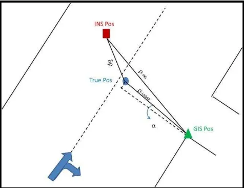
Several approaches for fusing INS with lidar have been considered. Here, we propose a fusion methodology, which is based on detection of building corners from the lidar data for buildings with a known position (e.g., ground plan information). With such information at hand, an approximation of the unknown actual vehicle position may be obtained and utilized as a position aiding to the INS.

Figure 1: A corner detection scenario

where the calculated INS range defined from the INS position to the known detected corner is:



 

2



2

and the distance between the INS and the true position



 

2



2

t INS t INS

x

x

y

y

 







(9)

Then, the computed position pt



xt yt



is used as a position aiding to the INS. That is, the difference between the estimated INS position,p_INS, and the above-mentioned calculated position is used as the residual measurement,

INS t

zp p, in the Kalman Filter.

This relatively simple strategy enables turning the laser scanning related information into a reference/control information that is added into the navigation solution.

3 ANALYSIS AND DISCUSSION

To evaluate the proposed approach a simulated test of a

vehicle’s trajectory traveling in a constant velocity of 50 km/h for 60 seconds is studied. The elevation is set to a constant value throughout the trajectory. Laser ranging noise is considered having a std. of L0.05[ ]m . The INS contains an

Inertial Measurement Unit (IMU) with a classical implementation of a triad of accelerometers and gyros. It is assumed that the accelerometer and gyro measurements contain only of white noise with a std. of end, the following error measure is utilized:

( )

( )

( )

velocity errors are obtained from

 

2

 

2

 

2 between two successive crossing detections. These detections are translated into two successive measurements. We consider the time between two successive measurements to be 5 seconds. The filter functions then in a prediction mode for the next 5 seconds until the following measurement is provided. For simplicity, the time between two consecutive measurements remains constant throughout the trajectory. The results of such aiding are presented in Figure 2 for position

Time between Measurements: 5 [sec]

LIDAR Aiding Standalone INS

0 10 20 30 40 50 60

Time between Measurements: 5 [sec]

LIDAR Aiding Standalone INS

Figure 3: Velocity error for lidar aiding versus standalone INS.

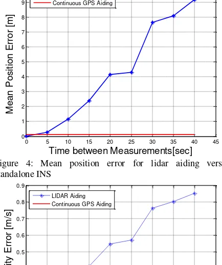
As Figure 2 shows, the standalone INS position solution drifts, and after 60 seconds has an error of about 80 meters. When applying laser scanning data as an aiding, at a 5 seconds interval, the INS drift drops dramatically and the combined solution is bounded by a maximal error which is lower than 0.4 meter, and even lower on average. Notice that this performance was obtained with only twelve measurements (at a 5 seconds interval). The same behavior occurs with the velocity error, where the standalone INS drifts and has an error of 3.3 m/s after 60 seconds, while the lidar aiding solution has a bounded error of 0.4 m/s and an average error of 0.15 m/s after 60 seconds. It follows that such aiding greatly improves the standalone INS solution and reaches a bounded solution for both position and velocity vectors.

To examine the proposed approach further, we use the same trajectory but with different time intervals between two measurements. The intervals vary from 0.05 seconds (equaling the INS sampling rate), to 40 seconds. The number of measurements throughout the trajectory varies accordingly from 1 (40 seconds) to 1200 (0.05 seconds). For each period, performance is. A comparison that is made for the performance of the aided INS to the fusion between GPS/INS while assuming GPS is continuously available is also shown in both figures. It is shown that when the time interval is of 5 seconds, the performance is almost equivalent to the one achieved by the GPS/INS integration. Thus, availability on ground plans as landmarks and the derivation of equivalent information (e.g., building corners, but other objects as well) from the laser scanning data can contribute to securing the accuracy-level of the mapping data in such zones.

4 CONCLUSIONS

This paper explored the possibility of using lidar measurements as aiding by using detected crossing between buildings. Employing the proposed methodology, crossing data are translated into positional information, which are then used

as aiding to the INS. Simulation results of such fusion showed improvements relative to the standalone INS performance in estimating the position and velocity components. Other than applying the proposed methodology on actual data, future research, will also address cases of partial GPS availability and utilize this information into the proposed methodology.

0 5 10 15 20 25 30 35 40 45

Figure 5: Mean velocity error for lidar aiding versus standalone INS

5 REFERENCES

Brandit, A. and Gardner, J., F., Constrained navigation algorithm for strapdown inertial navigation systems with reduced set of sensors, Proceedings of the American control conference pp. 1848-1852, Philadelphia PA., 1998.

Dissanayake, G., Sukkarieh, S., Nebot, E. and Durrant-Whyte, H., The aiding of a low cost strapdown inertial measurement unit using vehicle model constraints for land vehicle applications, IEEE transactions on robotics and automation, 17 (5), pp. 731-747, 2001.

El-Sheimy, N., Andel-Hamid, W. and Lachaplle, G., An adaptive neuro fuzzy model for bridging GPS outages in MEMS-IMU/GPS land vehicle navigation, in Proceeding of the ION GNSS, pp. 1088-1095, Long Beach, California, 2004.

integrated system in urban canyons, in Proceedings of ION GPS, Long Beach, CA, U. S. Institute of Navigation, Fairfax VA, September 2005, pp. 1977-1990.

Klein I, Filin S and Toledo T, Pseudo-measurements as aiding to INS during GPS outages, Navigation: Journal of the Institute of Navigation, 57(1), pp 25-34, 2010.

Maybeck P. S., Stochastic models, estimation and control, Volume 1, Navtech Book & Software store, 1994.

Pfister S., Roumeliotis S., Burdick J., Weighted Line Fitting Algorithms for Mobile Robot Map Building and Efficient Data Representation. in Proceedings of the IEEE International Conference on Robotics and Automation, 2003.

Shin, E.-H., Estimation Techniques for low-cost inertial navigation, UCGE reports number 20219, the University of Calgary, Calgary, Alberta, Canada, 2005.

Soloviev, A., Bates, D., van Graas, F, Tight Coupling of Laser Scanner and Inertial Measurements for a Fully Autonomous Relative Navigation Solution", NAVIGATION, Vol. 54, No. 3, Fall pp. 189-205, 2007. Soloviev, A. and de Haag M. U., Three-dimensional

navigation with scanning LiDARs: concept & initial verification, IEEE transactions on Aerospace and Electronic System, Vol. 36, No.1, pp. 14-31, 2010.

Stephen, J. and Lachapelle, G., Development and testing of a GPS-augmented multi-sensor vehicle navigation system. The journal of navigation, Vol. 54(2), pp. 297-319, 2001.

Titterton, D., H. and Weston, J., L., Strapdown inertial navigation technology – second edition, The American Institute of Aeronautics and Astronautics and the institution of electrical engineers, 2004.

Zarchan, P. and Musoff, H., Fundamentals of Kalman filtering: a practical approach second edition, The American Institute of Aeronautics and Astronautics, 2005.

6 APPENDIX – A

( ) 1

ˆ

ˆ

,

F t t

k k

x

_

 

x



 

e



(B.1)

1

T

k k k

P

_

   

P



Q

(B.2)

where the superscripts – and + represent the predicted and updated quantities (before and after the measurement update, respectively); x and

P

are the system state and the associated error covariance matrices respectively;



is the state transition matrix from time k to time k+1;

F t

( )

is the system dynamics matrix; and

Q

_k is the process-noise covariance-matrix (Maybeck 1994) given by:

     

     

1 2

T T T

k k k k k k k k k

Q  _G t Q t G t G t Q t G t  _ t

(B.3)

where, G t( )is the shaping matrix, and t is the time step.

The update is implemented by:





1

1 1 1 1 1 1 1

T T

k k k k k k k

K

_



P H

_{ }

H

_

P H

_{ }



R

_ 

(B.4)





1 1 1 1 1 1

ˆ

k

ˆ

k k k k

ˆ

k

x

_



x

_



K

_

z

_



H

_

x

_

(B.5)





1 1 1 1

k k k k

P

_



I



K

_

H

_

P

_

(B.6)

where

K

_kis the Kalman gain;

H

_kis the measurement matrix;

k