PIXEL-BY-PIXEL ESTIMATION OF SCENE MOTION IN VIDEO
A. G. Tashlinskii a*, P. V. Smirnov a, M. G. Tsaryov a
a Ulyanovsk State Technical University, Radio Engineering Faculty, Severnyi Venets str., 32, Ulyanovsk, 432027 Russia -
[email protected], [email protected], [email protected]
Commission II, WG II/5
KEY WORDS: video sequence, image processing, moving object detection, tracking, recurrent procedures, reverse processing
ABSTRACT:
The paper considers the effectiveness of motion estimation in video using pixel-by-pixel recurrent algorithms. The algorithms use stochastic gradient decent to find inter-frame shifts of all pixels of a frame. These vectors form shift vectors’ field. As estimated parameters of the vectors the paper studies their projections and polar parameters. It considers two methods for estimating shift vectors’ field.The first method uses stochastic gradient descent algorithm to sequentially process all nodes of the image row-by-row. It processes each row bidirectionally i.e. from the left to the right and from the right to the left. Subsequent joint processing of the results allows compensating inertia of the recursive estimation. The second method uses correlation between rows to increase processing efficiency.It processes rows one after the other with the change in direction after each row and uses obtained values to form resulting estimate. The paper studies two criteria of its formation: gradient estimation minimum and correlation coefficient maximum. The paper gives examples of experimental results of pixel-by-pixel estimation for a video with a moving object and estimation of a moving object trajectory using shift vectors’ field.
* Corresponding author
1. INTRODUCTION
One of the challenges in video processing is moving object detection and tracking. Some tasks require only detection of the motion, while others – extraction of the moving object or the motion area boundary. The biggest challenge is to estimate parameters of the object motion in video sequence. A solution quality to the problem largely depends on the accuracy of moving object area detection, since all the information needed to determine motion parameters and trajectory of the object is extracted from the image.
There are various approaches to identify area of moving object based on the interframe difference (Elhabian, 2008, Karasulu, 2013), background subtraction (Elhabian, 2008, Wang, 2010), the use of statistics (Karasulu, 2013, Kuczov, 2006), block estimation (Grishin, 2008), optical flow analysis (Zoloty’kh, 2012). The processing can be presented as estimation of inter-frame geometric deformations of two images, one of which can be considered as the reference image
irjr
z,
Z and the second
as deformed image Zd
zid,j in the image sequence
tj i t
z,
Z , where t – a number of a frame; t j i
z, – brightness of the image node with coordinates
i,j .Let H
hi,j be an inter-frame shift vectors’ field for all thenodes
i,j of reference image corresponding to the deformed image. The shift vector can be represented as its projections hxand hy or in polar form using its length i,j and angle i,j
with respect to the x axis. The parameters (hx,hy) and (,) are functionally equivalent. However, due to the inertia of recurrent estimation of shift vectors’ field H estimates for the
sets of parameters (hx,hy) and (,), are different since they have different physical meaning (Smirnov, 2015). The answer to the question of which set is preferable for solving the problem of moving object area detection is not obvious and requires research.
2. ESTIMATION ALGORITHMS
The technique for estimating shift vectors’ field H is proposed. Stochastic gradient descent algorithm (Tashlinskii. 2007) sequentially estimates the parameters i,j of shift vectors for all
the points
i,j of the image Zr:
ij ji j
i, 1 ˆ, signβ ,
ˆ
Λ , (1)
where Λ – the matrix of learning rates, which determines the rate of change of the estimated parameters
β – gradient estimation of an objective function.
The algorithm uses a reverse processing (Tashlinskii, 2013). It processes each row i bidirectionally: first, from the left to the right:
ˆ sign ˆ ,
ˆ
, ˆ sign ˆ
ˆ
, ,
1 ,
, ,
1 ,
j i hy h l
y j i l
y j i
j i x h l
x j i l
x j i
h h
h
h h
h
(2)
getting the estimates αˆil,j, and then from the right to the left
getting the estimates αˆir,j:
function because the brightness of adjacent frames changes slightly. Then using parameters (hx,hy) gradient estimation can be written as follows:
r
obtained from Zd by means of interpolation
d
. Otherwise, set of possible values of
the estimate ˆi,j is given by: two criteria (Tashlinskii, 2015): gradient estimation minimum:
and correlation coefficient maximum:
inertia of the recursive estimation. A comparative efficiency analysis has shown that the accuracy is higher (as well as computational cost) for correlation coefficient maximum. In the approach discussed above images are processed, in fact, as one-dimensional signals. Taking into account correlation between rows we can improve the performance of the algorithm. To do this, rows are processed one after the other with change in direction after each row with the subsequent joint processing
of the estimates (ˆi,j1,ˆi,j) and (hˆi,j1,hˆi,j) of adjacent rows.
3. ANALYSIS OF EFFICIENCY
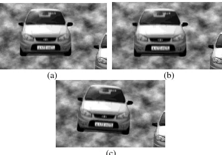
To analyze the efficiency of the algorithms we used images shown in Fig. 1. These are adjacent frames of a video sequence where the vehicle located in the center is moving and the vehicle on the right is motionless. The parameters of inter-frame spatial shift of the moving vehicle are hx3, hy2.95 for
Figure 1. An example of adjacent frames of a video sequnce with a moving object
3.1 Formation of shift vectors’ field
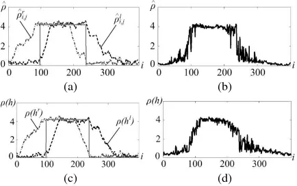
Fig. 2 shows typical results of shift magnitude estimation for a single row of a reference image while using criterion (6). For a
correct comparison, estimates (hˆ i,jx,hˆ i,jy) are recalculated to
lh
and
hr on i and Fig. 2(d) – the result of their jointprocessing. Solid grey line represents the true value of the deformation parameter.
The results for parameters (,) are visually better. Estimates given in Table 1 also confirm that. Table 1 shows mean value
h
m and variance 2h of estimation error for a processed row
using criterion (6). Estimation errors are presented for motion area and for area without motion. Note that the mean value and the variance of estimation error for the motion area are less for parameters (,). Parameters (,) are also preferable for the area without motion due to the lower bias of estimates despite slightly higher variance.
(a) (b)
(c) (d)
Figure 2. Estimates of the parameters for a row using criterion (6)
Fig. 3 shows the results of joint processing for the same row using criterion (7). Results in Fig. 3(a) correspond to the set of parameters (hx,hy), Fig. 3(b) – (,). Table 1 summarizes numerical characteristics of estimation errors for the row and for the entire image.
(a) (b) Figure 3. Estimates of the parameters for a row
using criterion (7)
Fig. 4 shows the results of joint processing of adjacent rows (algorithms C and D). Fig. 4(a) corresponds to the set of parameters (hx,hy), Fig. 4(b) – (,). Criterion (6) is used. Fig. 4(c) and Fig. 4(d) show results for the sets of parameters
) ,
(hx hy and (,) respectively. Criterion (7) is used. Fig. 4
shows that the use of correlation between rows significantly improves the results of parameters estimation compared to reverse processing of a single row.
(a) (b)
(c) (d)
Figure 4. Estimates of the parameters for a joint processing of adjacent rows
For the parameters (hx,hy) and criterion (6) mean value of the error for motion area decreases by 1.2 times, error variance – by 1.1 times, and for the criterion (7) – by 3 times and 20 times respectively. For the set of parameters (,) and criterion (6) mean value of the error for motion area decreases by 5 times, variance – by 2.1 times, and for the criterion (7) – by 10 times and 2.5 times respectively. Table 1 shows the actual values.
Algorithm
Motion area Area without motion
h
m h2102 mh
2 2
10
h
A 0,28 4,8 0,28 1,9
B 0,21 1,53 0,15 0,74
C 0,06 0,61 0,07 0,27
D 0,04 0,54 0,01 0,02
Table 1. Estimation error of shift vectors’ field for a row
The comparison of the algorithms with a well-known block algorithm MVFAST (Motion Vector Field Adaptive Search Technique) shows that MVFAST has worse accuracy of moving object detection in equal conditions. Moreover, MVFAST does not allow to get sub-pixel accuracy. Table 2 shows mean value and variance of estimation error for areas with and without motion for the entire image. It contains the results both for MVFAST and proposed algorithms.
Algorithm
Motion area Area without motion
h
m h2102 mh
2 2
10
h
A 0,42 7,3 0,29 2,6
B 0,34 1,47 0,15 1,35
C 0,07 1,24 0,09 0,28
D 0,01 0,69 0,02 0,02
MVFAST 0,08 18,6 0,02 0,05
Table 2. Estimation error of shift vectors’ field
Fig. 5 shows visualization of estimates of shift vectors’ field H for the reverse processing algorithms. Fig. 5 shows the magnitudes of the estimated vectors as a function of node coordinates of the reference image. Fig. 5(a) and Fig. 5(b) show results for the set of parameters (hx,hy)and criteria (6) and (7) respectively. Fig. 5(c) and Fig. 5(d) – parameters (,) and criteria (6) and (7) respectively.
(a) (b)
(c) (d) Figure 5. Shift vectors’ field for reverse processing
Fig. 6 shows visualization of field H estimates for algorithms C and D. Fig. 6(a) and Fig. 6(b) correspond to the set of parameters (hx,hy) and criteria (6) and (7) respectively,
Fig. 6(c) and Fig. 6(d) – parameters
(
,
)
and criteria (6) and (7) respectively. Figures confirm and illustrate well the conclusions.
(a) (b)
(c) (d)
Figure 6. Shift vectors’ field for joint processing of adjacent rows
3.2 Moving object detection and tracking
Fig. 7 shows moving object area and its contour obtained from the results of algorithms C and D by thresholding with threshold equal to 0.1 of the maximum value of . Note that there are practically no errors of the second kind for the algorithm D.
Figure 7. Results of moving object area identification
The above results correspond to the analysis of frames in Fig. 1(a) and Fig. 1(b), which are characterized only by a parallel shift of the moving object. Fig. 8(a) and Fig. 8(b) show the
frames in Fig. 1(a) and Fig. 1(c) which are characterized by
shift h
2,3T and rotation by angle 4. After the motion area identification, it is not difficult to estimate the parameters of motion, described, for example, by a similaritymodel. Results for the algorithm C are hˆ
1.98,3.04
T,
08 . 4 ˆ
and scale factor equal to 1.002; for the algorithm
D: hˆ
1.77,2.61
T, ˆ3.3 and scale factor is 0.988. Note that the set of parameters (hx,hy) provides a higher accuracy due to lower inertia of the change in their estimates. At the same time, this set provides less accuracy of identification of moving object area.
(a) (b) Figure 8. Estimation of shift vectors’ field under rotation
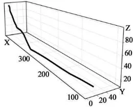
The object trajectory can be estimated using the field H. Fig. 9 shows two frames from a video of the landing to aircraft carrier and Fig. 10 shows the result of processing of 34 frames of the video. It shows the trajectory of the aircraft in relative coordinates XYZ. The camera position at the initial moment of the shooting is taken as the origin.
Figure 9. An example of frames of a video sequence
Figure 10. The tracking of the aircraft on the video sequence
A complicating factor in the example was the uneven camera movement toward the aircraft. Therefore, to estimate the position of the moving object relative to the scene (not to the camera) it was necessary not only to detect and identify the moving object area but also to stabilize the image.
4. CONCLUSION
The conducted studies showed that pixel-by-pixel stochastic gradient estimation of inter-frame shift vectors of all points of the reference image corresponding to its nodes (the shift vectors’ field) is an effective approach to solving the problem of finding motion of a scene in video sequence.
The estimated parameters of the shift vectors can be either their projections to the basic axis, or the polar parameters. Experimental studies have shown that the use of the polar parameters gives a greater accuracy of the shift vectors’ field and, accordingly, the identification of the motion area.
The paper presents and studies two methods of estimating shift vectors’ field. In the first method, stochastic gradient descent algorithm sequentially processes all nodes of the image row-by-row. Each row is processed bidirectionally. The joint processing of the estimates allows compensating inertia of the recursive procedure. However, this method does not consider correlation between adjacent rows and processes images as one-directional signal. The second method uses the correlation between rows to increase processing efficiency. The method processes rows one after the other with change in direction after each row and performs the joint processing of the estimates of adjacent rows. This approach shows significantly smaller estimation error of the field with roughly equal computational costs.
Two criteria of optimal estimates formation have been studied: minimum of gradient estimation of objective function and maximum of correlation coefficient of image’s local area. The latter criterion shows better results (but also higher computational cost). For this criterion, not only mean value and variance of estimation error are less, but there are also fewer oscillations in the area without motion.
Comparison of the proposed algorithms with the well-known block algorithm MVFAST (Motion Vector Field Adaptive Search Technique) has shown that MVFAST has worse accuracy of moving object detection under equal conditions. In addition, the proposed algorithms, in contrast to the MVFAST, make it possible to obtain a subpixel accuracy of estimation.
The conducted experiments confirmed that the proposed algorithms are efficient in finding moving object parameters (parallel shift, rotation angle and scale factor represent these parameters for the similarity model) and in estimating three-dimensional trajectory of a moving object using video sequence.
ACKNOWLEDGEMENTS
The reported study was funded by RFBR and Government of Ulyanovsk Region according to the research project № 16-41-732053, and the Russian Ministry of Education and Science, project no. 2017/232.
REFERENCES
Elhabian, Sh.Y., El-Sayed, Kh.M., Ahmed, S.H. 2008. “Moving Object Detection in Spatial Domain using Background Removal Techniques.” Recent Patents on Computer Science 1: 32-54. Grishin, S.V., Vatolin, D.S., Lukin, A.S. 2008. “The Block Methods Review of Motion Estimation in Digital Video
Signals.” Programmny’e sistemy’ i instrumenty’ 9: 50-62 [in Russian].
Karasulu, B., Korukoglu, S. 2013. Performance Evaluation Software: Moving Object Detection and Tracking in Videos. New York: SpringerBriefs in Computer Science.
Kuczov, R.V., Trifonov, A.P. 2006. “Moving Object Detection Algorithms in Image.” Izvestiya RAN. Teoriya i sistemy’ upravleniya 3: 129-138 [in Russian].
Smirnov, P.V., Tashlinskii A.G. 2015. “Method for Moving Object Area Identification in Image Sequence.” Radiotekhnika
6: 5-11 [in Russian].
Tashlinskii, A.G. 2007. “Pseudogradient Estimation of Digital Images Interframe Geometrical Deformations.” Vision Systems: Segmentation & Pattern Recognition. Vienna, Austria: I-Tech: 465-494.
Tashlinskii, A.G., Kurbanaliev, R.M., Zhukov, S.S. 2013. “Method for detecting instability and recovery of signal shape under intense noise.” Pattern recognition and image analysis 23 (3): 425-428.
Tashlinskii, A.G., Smirnov, P.V. 2015. “Moving Object Area Identification in Image Sequence.” International Siberian Conference on Control and Communications, IEEE Conference
№ 35463. 10.1109/SIBCON. 2015.7147239.
Wang, L., Yung, N.H.C. 2010. “Extraction of Moving Objects from Their Background Based on mulitple adaptive threshold and boundary evaluation.” IEEE Trans. Intelligent transportation systems 11: 40–51.
Zoloty’h, N.Yu., Kustikova, V.D., Meerov, I.B. 2012. “The Review of Searching and Tracking Methods in Video.” Vestnik Nizhegorodskogo universiteta im. N.I. Lobachevskogo 5 (2): 348-358 [in Russian].