isprsarchives XXXIX B1 285 2012

INTERIOR ORIENTATION ERROR MODELLING AND CORRECTION

FOR PRECISE GEOREFERENCING OF SATELLITE IMAGERY

Chunsun Zhang, Clive S. Fraser

Cooperative Research Centre for Spatial Information, Dept. of Infrastructure Engineering, University of Melbourne, Australia - (chunsunz, c.fraser)@unimelb.edu.au

Shijie Liu

Department of Surveying and Geoinfomatics, Tongji University, Shanghai 200092, China liusjtj@gmail.com

Commission I, WG I/4

KEY WORDS: High resolution, Satellite, Sensor, Imagery, Orientation, Modelling, Georeferencing, Accuracy

ABSTRACT:

To exploit full metric quality of optical satellite imagery, precise georeferencing is necessary. A number of sensor orientation models designed to exploit the full metric potential of images have been developed over the past decades. In particular, generic models attract more interest as they take full account of the physical imaging process by adopting time dependant satellite orbit models and interior orientation (IO) information provided by the satellite imagery vendors. The quality of IO parameters varies for different satellites and has significant impact on the georeferencing performance. Self-calibration approaches have been developed, however such approaches require a significant amount of ground control with good point distribution. In addition, the results are not always stable due to the correlation between the model parameters. In this paper, a simple yet efficient method has been proposed to correct the IO errors by detailed examination and efficient modelling of the IO error distribution in the focal plane. The proposed correction method, used in conjunction with a generic sensor model, significantly improves the metric performance of satellite images, leading to sub-pixel georeferencing accuracy.

1. INTRODUCTION

High-resolution satellite imagery (HRSI) with a spatial resolution of 2.5m or greater is becoming increasingly accessible to the mapping and GIS community, and along with high spatial resolution comes the challenge of dimensionally characterising the earth’s surface to finer detail with higher accuracy and reliability. To exploit full metric quality of optical satellite imagery and precise georeferencing, a number of sensor orientation models have been developed over the past three decades. These have ranged from empirical models, through to camera replacement models such as the now popular rational function model (Fraser and Hanley, 2003; Fraser et al., 2005), and to rigorous parametric formulations which model the physical image-to-object space transformation (Kratky, 1989; Westin, 1990; Chen and Lee, 1993; Dowman and Michalis, 2003; Poli, 2005; Kim and Dowman, 2006). In the case of vendor supplied rational polynomial coefficients (RPCs), it has been well established that there need be no loss in georeferencing accuracy when bias-corrected RPCs are employed (Fraser and Hanley, 2003; Fraser et al., 2005).

Generic models attract more interest as they take full account of the physical imaging process by adopting time dependant satellite orbit models and interior orientation (IO) information provided by the satellite imagery vendors. Moreover, given the increasing number of HRSI satellites being deployed, the attraction of a generic sensor orientation model suited to a wide range of satellite imagery becomes compelling. In aiming to develop a more generic sensor model, Weser et al. (2008a; 2008b) adopted cubic splines to model the satellite trajectory and the sensor attitude. The advantage of the physical model is that it is flexible in that it can be readily adapted to most HRSI

vendor-specific definitions for sensor orientation. The compensation of systematic errors inherent in vendor-supplied orientation data is achieved through a least-squares sensor orientation adjustment, which incorporates additional parameters for bias compensation and employs a modest number of ground control points (GCPs).

One of the key components in a generic sensor model is interior orientation which is usually provided by the satellite imagery vendors. The quality of IO parameters varies for different satellites and has significant impact on the georeferencing performance. Self-calibration approaches have been developed and are efficient and powerful technique used for the calibration of photogrammetric imaging systems to determine the IO parameters. Usually, additional parameters are used to model systematic errors. They are defined in accordance with the physical structure of the imaging sensors. For orientation and calibration of ALOS/PRISM imagery, Kocaman and Gruen (2008) employed ten additional parameters for the interior orientation of each of three cameras to account for the scale and blending effects as well as the displacements of the centres of the CCD chips from the principal point. An affine model was presented in Weser et al. (2008) to compensate for the displacement of the relative positions of the CCD chips. The model parameters are determined in the sensor orientation adjustment process. While these methods have demonstrated efficiency in georeferencing of satellite imagery, however, self-calibration approaches require a significant amount of ground control points. In addition, the performance is highly influenced by the distribution of GCPs. Moreover, the results are not always stable due to the correlation between the model parameters. Full set of radial and tangential distortion parameters are difficult to address, and the appropriate International Archives of the Photogrammetry, Remote Sensing and Spatial Information Sciences, Volume XXXIX-B1, 2012

parameters have to be selected based on the analysis of their correlations and quality (Radhadevi et al., 2011).

In this paper, a simple yet efficient method has been proposed to correct the IO errors by detailed examination and efficient modelling of the IO error distribution in the focal plane. The research has been carried out within a generic sensor model developed at the University of Melbourne, which has been successfully applied to a number of satellite sensors. Imagery acquired from FORMOSAT-2 and THEOS satellites are used to illustrate the modelling procedures. In the following section, the generic sensor orientation model is briefly reviewed. This is followed by a discussion of an IO correction model that was found to compensate apparent errors in the provided sensor IO parameters. Finally, the conduct and results of the experimental validation of the IO correction model in georeferencing for THEOS and FORMOSAT-2 data sets are presented and concluding remarks are offered.

2. GENERIC SENSOR ORIENTATION MODEL Thegeneric sensor model adopted, which was developed within the Cooperative Research Centre for Spatial Information, has previously been successfully applied to a number of current HRSI systems, including WorldView-1 and -2, QuickBird, SPOT5, Cartosat-1, ALOS PRISM and THEOS (Weser at al., 2008a, 2008b; Fraser at al., 2007; Rottensteiner et al., 2009; Liu et al., 2011). A short overview of the model will be presented here; full details about the generic sensor model and accommodation of each HRSI system can be found in Weser et al. (2008a, 2008b).

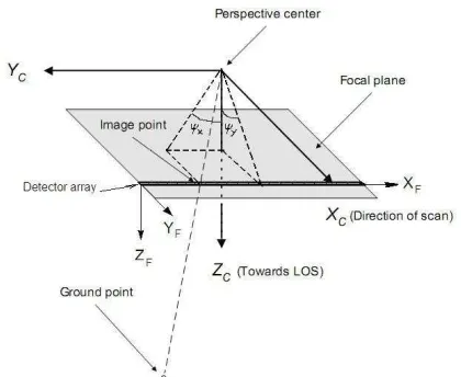
The physical model for a pushbroom satellite imaging sensor, which relates an object point PECS in an earth-centered object coordinate system to the position of its projection PI = (xI, yI, 0)Tin the image plane coordinate system, is expressed as

( )

t R R

( )

t

[

C R

(

p c x

)

]

S

P_ECS= + _O⋅ _P ⋅ _M +

λ

⋅ _M⋅ _F− _F+

δ

(1)

The coordinate yI of an observed image point directly corresponds with the recording time t for the image row through t = t0 + ∆t · yI, wheret0 being the acquisition time of the first image line and ∆t the time interval between scans. PF = (xI, 0, 0)Trefers to an individual CCD array. The vector cF in Eq.1 represents the position of the projection centre in the detector coordinate system, and

δ

x

formally describes the image biases (eg refraction and residual systematic errors). The rotation matrix RM and shift CM describe the rigid motion of the camera with respect to the satellite platform. They are referred to as the camera mounting parameters. The satellite orbit path is modelled by time-dependant functions S(t). The time-constant rotation matrix RO rotates from the earth-centred coordinate system to a system defined at the scene centre tangent to the orbit path. It can be computed from the satellite position and velocity at the scene centre. The time-dependent rotation matrix Rp(t) rotates from the defined orbit system to the satellite platform system, and it is formed from three time-dependent rotation angles: roll, pitch and yaw. The components of the orbit path and the time-dependant rotation angles are in turn modelled by cubic spline functions.

The coefficients of the spline function are initialised from the orbit and attitude data recorded on board the satellite. Afterwards, the sensor orientation adjustment is performed to compensate for systematic errors, with observations of image points, GCPs, orbit point coordinates and observed rotations.

The adjusted parameters then enable precise determination of the exterior orientation of the image(s). Further details of the sensor orientation adjustment process can be found in Weser et al. (2008a, 2008b).

The generic sensor orientation model can also treat a continuous strip of images recorded in the same orbit. Under this approach, which does not require the measurement of tie/pass points, the orbit path and attitude data for each separate scene of a strip are merged to produce a single, continuous set of orbit and attitude observations, such that the entire strip of images can be treated as a single image, even though the separate scenes are not merged per se (Rottensteiner et al., 2009; Fraser and Ravanbakhsh, 2010). As a result, the number of unknown orientation parameters is considerably reduced, and so also is the amount of ground control, which can then be as little as two GCPs at each end of the strip.

3. MODELING AND CORRECTION OF IO ERRORS 3.1 Modelling of Interior Orientation

The IO parameters describe the position of the projection center in the framelet coordinate system. For THEOS and FORMOSAT-2, the IO parameters are available indirectly through two orthogonal view angles x and y to each pixel in

The relationship between each pixel i in the linear array and the view angles can be described as

−

International Archives of the Photogrammetry, Remote Sensing and Spatial Information Sciences, Volume XXXIX-B1, 2012

Here, rij is the element of the rotation matrix calculated from the points lie on a straight line, the rotation angle about the XF axis, which cannot be determined, is assigned a constant value of zero. Because of the high correlation between the rotation angles and the offsets, e.g. roll is highly correlated with x0 and pitch with y0, the normal equation system of the least-squares adjustment would be ill-conditioned, leading to the potential recovery of erroneous values for the parameters. Weighted constraints can be applied to alleviate this problem, for example the angle pitch can be constrained to a near-zero value.

3.2 Correction of IO errors

The quality of IO estimation relies on the precision of the line-of-sight data. Errors in these data result in poor quality of IO parameters, which in turn degrade the geometric potential of the imagery. Thus, corrections to interior orientation should be performed before precise georeferencing can be conducted. Additional parameters have been extensively used in photogrammetric mapping systems to improve the sensor’s interior orientation parameters and to model other systematic errors. The additional parameters and the correction models should be chosen carefully in accordance with the physical structure of the sensors. In general, compensation of errors in IO parameters can be achieved via polynomial correction functions: provided cubic polynomial coefficients. Afterwards, an initial determination of the IO parameters and detector mounting rotations is made which enables examination of the IO errors rotation angles of THEOS imagery.

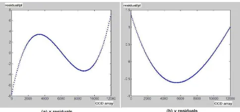
The estimated value of x0shown in Table 1 indicates that the perspective centre lay within a pixel of the centre of the 12,000-pixel linear array, and the view angles provided in the metadata were symmetric about the array centre. It is noteworthy that whereas the residuals in the y coordinate (flight direction) were generally of a magnitude of less than 0.5 pixels, they grew to 1 pixel at the end regions of the detector. The residuals in x, on the other hand, reached 7 pixels at the two ends of the detector as illustrated in Figure 2. The large residual values encountered suggested either the presence of errors in the provided look angles or imprecise detector alignment within the CCD array, the former being a more plausible assumption. It can be seen from Figure 2 that the residuals are distributed symmetrically about the centre of the linear array. Whereas y-residuals show a parabolic distribution, the distribution for x-residuals is more complex, with more than 90% of values being beyond 1 pixel.

Figure 2. Residuals of IO estimation for THEOS imagery.

Similarly, the IO values were obtained from FORMOSAT-2 sensor. The residual distribution is presented in Figure 3. Again, the symmetrical pattern is observed. The residuals in x direction demonstrate a similar distribution as in THEOS, and are significantly larger than those in y direction, reaching 7 pixels at the both ends of the detector. While the distribution of the y -residuals is more complex than that in THEOS, the y-residuals are extremely small, with the largest value being around 0.02 pixels.

Figure 3. Residuals of IO estimation from provided view angles.

The symmetrical distribution of the IO residuals of the THEOS and FORMOSAT-2 satellite sensors indicate a behaviour International Archives of the Photogrammetry, Remote Sensing and Spatial Information Sciences, Volume XXXIX-B1, 2012

conducive to modelling via a cubic polynomials function. The coefficients a0 ~ a3 and b0 ~ b3 can be determined by least-squares estimation. The modelled residuals are then applied to the image measurements to compensate for IO errors in the subsequent georeferencing.

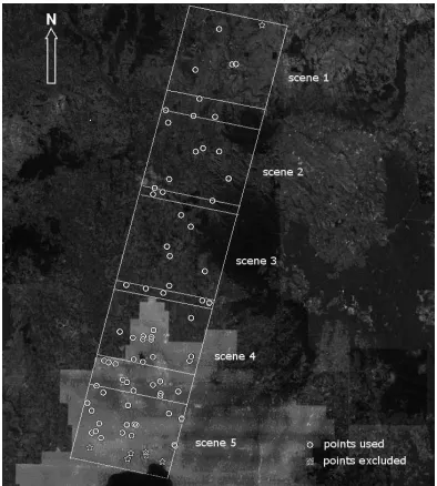
4. EXPERIMENTAL RESULTS AND DISCUSSION Experiments have been conducted to validate the efficiency of the proposed method for IO error modelling and correction. The THEOS test data comprised a strip of five mono panchromatic images recorded within a single orbit on 21 July 2009. Each scene covered an area about 23km wide x 25km long, and the total strip length was 107km (there was an average 13% overlap between the successive scenes). The location of the image strip, which extended from the City of Melbourne to rural areas north of the city, is shown along with GCP/Checkpoint positions in Figure 4. Within the metadata, the number of orbit observation points outside the image strip was restricted to one before the first scene, whereas the final observation was prior to the last image line of the strip. Generally, for optimal application of the generic sensor model, orbit observations need to not only span the full strip, but also extend into the scenes immediately before the first image and after the last.

The topography of the Melbourne test field ranges from relatively flat terrain in the south, with elevations near sea-level, to undulating hilly county with heights up to around 400m in the middle and northern regions. Some sections comprise forest, which accounts to some degree for the uneven distribution of the 82 image-identifiable GCPs/Checkpoints that were surveyed to an accuracy of better than 0.2m. This is equivalent to better than 0.1 pixels at ground scale. Due to inadequate orbit observations at the two ends of the strip, some eight points at the strip extremities were excluded from the analysis, thus leaving 74 points, which mainly comprised road roundabouts or road intersections. Image point observations were performed in the Barista software system to an accuracy estimated at 0.3 – 0.5 pixel.

Figure 4. THEOS 5-image strip and distribution of GCPs in Melbourne test field.

The second data set comprises four scenes of FORMOSAT-2 imagery over an area in Taiwan. The image size of a standard scene is 23km x 24km when viewed at nadir. The ground sampling distance is around 2m. The object coordinates of the GCPs were acquired from topographic maps. The accuracy of the coordinates is estimated at 3m which is significantly lower compared with the GCPs of the THEOS data set in Melbourne test field.

In order to examine the impact on accuracy of the presence or absence of the applied polynomial correction function for the IO of THEOS imagery, two sets of sensor orientation adjustments were carried out, both utilizing all GCPs as error free observations. The results for the cases of with and without image coordinate correction are listed for each scene in Table 2.

Table 2. Image space residuals obtained in georeferencing of THEOS imagery with and without IO correction.

It is observed that significant improvements are obtained in modelling the IO within the x-coordinate direction (detector axis), resulting in RMS values of residuals dropping from around 2 pixels or larger down to 0.5 pixels or smaller. The correction in y coordinates, however, had no significant impact on the ultimate accuracy. This can be explained that most of the modelled residuals in y direction are less than half pixel, thus, the correction could probably be overwhelmed by the measurement error of the image coordinates. For the scenes 4 and 5, there are considerable amount of points located in the marginal area where the magnitude of the correction in y is around one pixel (see Figure 4). As a result, larger corrections are applied and more improvement in y direction are attained for these two scenes, as can be seen in the last two rows of Table 2.

The performance of the IO error modelling and correction approach on FORMOSAT-2 imagery is presented in Table 3. Similar to the case of THEOS imagery, large improvements has been achieved in x–coordinate direction. The RMS values dropped from over 3 pixels to less than 2 pixels with IO correction. Little or no improvement was observed in y -coordinate direction. This is due to the extremely small residuals in the flight direction as shown in Figure 3, resulting in limited corrections in y-coordinate direction.

Scene ID

Number of GCPs

Without image correction (pixel)

With image correction (pixel)

RMSx RMSy RMSx RMSy

Scene 1 84 3.225 3.174 1.462 3.172

Scene 2 170 3.321 4.462 1.889 4.463

Scene 3 120 3.384 2.647 1.940 2.642

Scene 4 157 3.417 2.599 1.952 2.599

Table 3. Image space residuals obtained in georeferencing of FORMOSAT-2 imagery with and without IO correction.

Scene ID Number of GCPs

Without image correction (pixel)

With image correction (pixel)

RMS x RMS y RMS x RMS y

Scene 1 8 2.72 0.36 0.21 0.36

Scene 2 13 2.33 0.31 0.26 0.33

Scene 3 16 1.89 0.42 0.39 0.28

Scene 4 32 1.99 0.49 0.35 0.34

Scene 5 29 2.83 0.48 0.30 0.27

Compared with the THEOS imagery, the georeferencing accuracy of FORMOSAT-2 images is relatively low in this investigation. Notice the accuracy of the GCPs is estimated at 3m. This is not comparable with the GCPs used in THEOS imagery where the accuracy of the GCPs is better than 0.2m. It can be expected that with better quality of GCPs, higher georeferencing accuracy can be achieved from FORMOSAT-2 imagery.

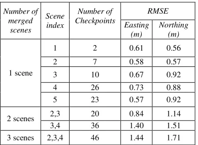
Further experiments was conducted to investigate the efficiency of the IO error modelling and correction approach within the generic sensor model for 2D georeferencing of THEOS imagery over the Melbourne test field with a few GCPs. Sensor orientation adjustments were performed for both single images and image strips. As explained earlier, due to inadequate orbit observation points in the metadata, strips formed by two or three consecutive images (excluding the first and last image) were examined. From this series of adjustments with configurations of 6 GCPs an estimate of planimetric georeferencing accuracy could be made based on the 2D residuals at ground checkpoints. The resulting planimetric checkpoint RMSE values are listed in Table 4.

Table 4. THEOS planimetric georeferencing accuracy expressed via RMS discrepancies at ground checkpoints.

The RMSE values in Table 4 provide representative measures of the external accuracy for 2D georeferencing from THEOS. It should be recalled that these arise from single configurations of 6 GCPs and variations in checkpoint discrepancy values can be expected with different control point configurations. It is noted in Table 4 that sub-pixel accuracy is achieved in all cases, even in the multi-scene configurations, although accuracy in these instances is lower than that achieved for the relatively more controlled single images.

5. CONCLUSION

This paper has presented an efficient approach for modelling and correction of IO errors in high-resolution satellite imaging sensor for precise georeferencing. An initial determination of IO parameters was made using the vendor-provided view angles. The residuals were then examined carefully to analyse the IO errors and their distribution in the focal plane for THEOS and FORMOSAT-2 sensors. It turns out the IO errors can be compensated for via third-order polynomial functions, the coefficients being determined by least-squares estimation based on the residual distribution. As a result, x-image coordinate residuals could be reduced from 2 pixels RMS to sub-pixel level in THEOS imagery, leading to sub-pixel georeferencing accuracy. With the IO error modelling and correction, the magnitude of the RMS values in FORMOSAT-2 dropped from over 3 pixels to less than 2 pixels. While this improvement is

not as significant as in the case of THEOS imagery, it is worth to note this georeferencing performance is achieved using GCPs of 3m accuracy. Better geometric performance of FORMOSAT-2 imagery can be expected if GCPs with higher accuracy are available. In Melbourne test field, application of IO error modelling and correction approach within the generic sensor model has yielded sub-pixel (0.5 to 2m) 2D georeferencing accuracy in THEOS 3-image strip adjustments utilising only six GCPs. In conclusion, the experimental results demonstrate that the proposed modelling approach can efficiently account for the IO errors caused by the imprecise metadata supplied by the satellite imagery vendors, therefore, significantly improving the geometric performance of the high-resolution satellite imagery.

6. REFERENCES

Chen, L.C. and Lee, L.-H., 1993. Rigorous generation of digital orthophotos from SPOT images. Photogrammetric Engineering and Remote Sensing, 59(5): 655-661.

Dowman, I. and Michalis, P., 2003. Generic rigorous model for along track stereo satellite sensors. Proceedings of Joint Workshop on High Resolution Mapping from Space (Eds. M. Schroeder, K. Jacobsen & C, Heipke), 6 – 8 October, Hanover, Germany. 6 pages on CD-ROM.

Kratky, V., 1989. Rigorous photogrammetric processing of SPOT images at CCM Canada. ISPRS Journal of Photogrammetry and Remote Sensing, 44(2): 53–71.

Fraser, C.S. and Hanley H.B., 2003. Bias compensation in rational functions for IKONOS satellite imagery. Photogrammetric Engineering and Remote Sensing, 69(1): 53-57.

Fraser, C.S., Rottensteiner, F., Weser, T. and Willneff, J., 2007. Application of a generic sensor orientation model to SPOT 5, QuickBird and ALOS Imagery. Proceedings of 28th Asian Conference on Remote Sensing, 12-16 November, Kuala Lumpur. 7 pages on CD-ROM.

Fraser, C.S. and Ravanbakhsh, M., 2010. Precise georeferencing of long strips of ALOS imagery. Photogrammetric Engineering and Remote Sensing, 77(1): 87-93.

Kim, T. and Dowman, I., 2006. Comparison of two physical sensor models for satellite images: Position-Rotation model and Orbit-Attitude model. Photogrammetric Record, 21(114): 110-123.

Kocaman, S. and Gruen, A. 2008. Geometric Modeling and Validation of ALOS/PRISM Imagery and Products. International Archives of Photogrammetry, Remote Sensing and Spatial Information Sciences, Beijing, China. Vol. XXXVI, Part 3: 12-18.

Liu, S., Fraser, C., Zhang, C., Ravanbakhsh, M. and Tong, X., 2011. Georeferencing performance of THEOS imagery. Photogrammetric Record, 26(134):250-262.

Radhadevi, P. V., Müller, R., d‘Angelo, P. and Reinartz, P. 2011. In-flight Geometric Calibration and Orientation of ALOS/PRISM Imagery with a Generic Sensor Model. Photogrammetric Engineering and Remote Sensing, 77(5): 531-538.

Number of merged

scenes Scene index

Number of Checkpoints

RMSE

Easting (m)

Northing (m)

1 scene

1 2 0.61 0.56

2 7 0.58 0.57

3 10 0.67 0.92

4 26 0.73 0.88

5 23 0.57 0.92

2 scenes 2,3 20 0.84 1.14

3,4 36 1.40 1.51

3 scenes 2,3,4 46 1.44 1.71

Rottensteiner, F., Weser, T., Lewis, A. and Fraser, C.S., 2009. A strip adjustment approach for precise georeferencing of ALOS imagery. IEEE Transaction on Geoscience and Remote Sensing, 47(12): 4083-4091.

Weser, T., Rottensteiner, F., Willneff, J., Poon J. and Fraser C.S., 2008a. Development and testing of a generic sensor model for pushbroom satellite imagery. Photogrammetric Record, 23(123): 255-274.

Weser, T., Rottensteiner, F., Willneff, J. and Fraser, C.S., 2008b. An improved pushbroom scanner model for precise georeferencing of ALOS PRISM imagery. International Archives of Photogrammetry, Remote Sensing and Spatial Information Sciences, Beijing, 37(B1-2): 723-730.

Westin, T., 1990. Precision rectification of SPOT imagery. Photogrammetric Engineering and Remote Sensing, 56(2): 247– 253.