AquaFarm: simulation and decision support for
aquaculture facility design and management
planning
Douglas H. Ernst
a,*, John P. Bolte
a, Shree S. Nath
baBiosystems Analysis Group,Department of Bioresource Engineering,Oregon State Uni
6ersity, Gilmore Hall 102B,Cor6allis,OR 97331, USA
bSkillings–Connolly,Inc.,5016 Lacy Boule
6ard S.E.,Lacy,WA 98503, USA
Received 20 September 1998; accepted 3 September 1999
Abstract
Development and application of a software product for aquaculture facility design and management planning are described (AquaFarm, Oregon State University©). AquaFarm provides: (1) simulation of physical, chemical, and biological unit processes; (2) simulation of facility and fish culture management; (3) compilation of facility resource and enterprise budgets; and (4) a graphical user interface and data management capabilities. These analytical tools are combined into an interactive, decision support system for the simulation, analysis, and evaluation of alternative design and management strategies. The quantitative methods and models used in AquaFarm are primarily adapted from the aquaculture science and engineering literature and mechanistic in nature. In addition, new methods have been developed and empirically based simplifications implemented as required to construct a comprehensive, practically oriented, system level, aquaculture simulator. In the use of AquaFarm, aquaculture production facilities can be of any design and management inten-sity, for purposes of broodfish maturation, egg incubation, and/or growout of finfish or crustaceans in cage, single pass, serial reuse, water recirculation, or solar-algae pond systems. The user has total control over all facility and management specifications, including site climate and water supplies, components and configurations of fish culture systems, fish and facility management strategies, unit costs of budget items, and production species and objectives (target fish weights/states and numbers at given future dates). In addition, parameters of unit process models are accessible to the user, including species-specific parameters of fish performance models. Based on these given specifications, aquaculture www.elsevier.nl/locate/aqua-online
* Corresponding author. Tel.: +1-541-7523917; fax:+1-541-7372082. E-mail address:[email protected] (D.H. Ernst)
122 D.H.Ernst et al./Aquacultural Engineering23 (2000) 121 – 179
facilities are simulated, resource requirements and enterprise budgets compiled, and opera-tion and management schedules determined so that fish producopera-tion objectives are achieved. When facility requirements or production objectives are found to be operationally or economically unacceptable, desired results are obtained through iterative design refinement. Facility performance is reported to the user as management schedules, summary reports, enterprise budgets, and tabular and graphical compilations of time-series data for unit process, fish, and water quality variables. Application of AquaFarm to various types of aquaculture systems is demonstrated. AquaFarm is applicable to a range of aquaculture interests, including education, development, and production. © 2000 Elsevier Science B.V. All rights reserved.
Keywords:Aquaculture; Decision support system; Computer; Design; Modeling; Simulation; Software
1. Introduction
Aquaculture facility design and management planning require expertise in a variety of disciplines and an ability to perform computationally intensive analyses. First, following specification of the physical, chemical, biological, and management processes used to represent a given facility, quantitative procedures are required to model these processes, project future facility performance, and determine facility operational constraints and capacities. Second, management of large datasets is often necessary, including facility and management specifications, projected facility performance and management schedules, and resource and economic budgets. Finally, design procedures require many calculations, especially when: (1) multiple fish lots and fish rearing units are considered; (2) simulation procedures are used to generate facility performance and management schedules; (3) alternative design and management strategies are compared; (4) designs are adjusted and optimized through a series of iterative facility performance tests; and (5) production econom-ics are compared over a range of production scales. Such analyses can be used to optimize production output with respect to required management intensity and resource consumption (or costs) and to explore tradeoffs between fish biomass densities maintained and fish production throughput achieved (residence time of fish in a facility).
by the development of simulation models for research purposes. Foretelling these trends, decision support systems have been developed for agriculture for purposes of market analysis, selection of crop cultivars, crop production, disease diagnosis, and pesticide application.
The purpose of this paper is to provide an overview of the development and
application of AquaFarm (Ver. 1.0, Microsoft Windows®, Oregon State
Univer-sity©). AquaFarm is a simulation and decision support software product for the design and management planning of finfish and crustacean aquaculture facilities (Ernst, 2000b). Major topics in this discussion are: (1) the division of aquaculture production systems into functional components and associated models, including unit processes, management procedures, and resource accounting; and (2) the flexible reintegration of these components into system-level simulation models and design procedures that are adaptable to various aquaculture system types and production objectives. To provide this overview at a reasonable length, methods and models of physical, chemical, and biological unit processes used in AquaFarm are presented as abbreviated summaries in an appendix to this paper. The appendix is organized according to domain experts and unit processes. Example applications of AquaFarm to typical design and planning problems are provided but rigorous case studies are beyond the scope of this paper. Completed and ongoing calibration and validation procedures for AquaFarm are discussed.
2. AquaFarm development
The aquaculture science and engineering literature was applicable to the develop-ment of AquaFarm through three major avenues. First, studies concerned with aquaculture unit processes and system performance provided models and modeling overviews for a wide range of physical, chemical, and biological unit processes and system types (Chen and Orlob, 1975; Muir, 1982; Bernard, 1983; Allen et al., 1984; James, 1984; Svirezhev et al., 1984; Cuenco et al., 1985a,b,c; Fritz, 1985; Tchobanoglous and Schroeder, 1985; Cuenco, 1989; Piedrahita, 1990; Brune and Tomasso, 1991; Colt and Orwicz, 1991b; McLean et al., 1991; Piedrahita, 1991; Weatherly et al., 1993; Timmons and Losordo, 1994; Wood et al., 1996; Piedrahita et al., 1997). Additional methods and models were newly developed for AquaFarm, including empirically based simplifications, as required to achieve comprehensive coverage of aquaculture system modeling while avoiding excessive levels of com-plexity and input data requirements. AquaFarm is primarily based on mechanistic principles, with empirical components added as necessary to support practically oriented design and management analyses for a wide range of users.
124 D.H.Ernst et al./Aquacultural Engineering23 (2000) 121 – 179
aquaculture educators, developers, and producers (Bourke et al., 1993; Lannan, 1993; Nath, 1996; Leung and El-Gayar, 1997; Piedrahita et al., 1997; Schulstad, 1997; Wilton et al., 1997; Stagnitti and Austin, 1998). These reported software applications range widely in their internal mechanisms and intended purpose. The software POND (Nath et al., 2000) is most similar to AquaFarm and some program modules have been jointly developed.
In the development of AquaFarm, it was desired to maintain a practical balance between the responsibilities required from users and the analytical capacity pro-vided by AquaFarm. These objectives are somewhat opposed, and a considerable level of user responsibility was found necessary to achieve desired levels of analysis. User responsibilities required in the use of AquaFarm consist of facility specifica-tions, model parameters, and decisions regarding alternative facility designs and management strategies. Facility specifications include items such as facility location (for generated climates) or climatic regimes (for file-based climates), source water variables, components and configurations of water transport, water treatment, and fish culture systems, management strategies, and production objectives. While approximate environmental conditions, typical facility configurations, and typical management strategies can be provided by AquaFarm, it is not possible to avoid user responsibility for these site-specific variables. In contrast, model parameters for passive unit processes (e.g. passive heat and gas transfer and biological processes) are ideally independent of site-specific conditions, given the use of sufficiently developed models. Validated, default values are provided for all parameters. However, due to the necessity of simplifying assumptions and aggregated processes in aquacultural modeling, model parameters may be dependent on site-specific conditions to some degree (Svirezhev et al., 1984). Thus, model parameters for passive unit processes have been made user accessible for any necessary adjustment. Finally, while the purpose of AquaFarm is to support design and management decisions, these decisions must still be made by the user. As a result, some level of user responsibility cannot be avoided regarding the underlying processes impacting system performance and implications of alternative decisions on facility perfor-mance and economics. Possible methods to alleviate user responsibilities are discussed in the conclusion to this paper.
AquaFarm is a stand-alone computer application, programmed in Borland
C+ +® and requiring a PC-based Microsoft Windows® operating environment.
The C+ + computer language was chosen for its popularity, portability,
availabil-ity of software developer tools, compatibilavailabil-ity with the chosen graphical user
interface (Microsoft Windows®), and support of object oriented programming
(OOP; Budd 1991; Nath et al., 2000). According to OOP methods, all components of AquaFarm are represented as program ‘objects’. These objects are used to represent abstract entities (e.g. dialog box templates) and real world entities (e.g. fish rearing units) and are organized into hierarchical structures. Each object contains data, local and inherited methods, and mechanisms to communicate with other objects as needed. The modular, structured program architecture supported by OOP is particularly suited to the development of complex system models such as AquaFarm.
3. AquaFarm design procedure
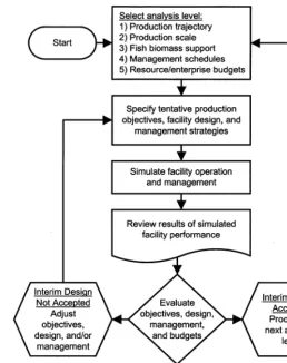
AquaFarm supports interactive design procedures, utilizing progressive levels of analysis complexity, simulation based analyses, and iterative design refinement (James, 1984e). These procedures are used to develop design and management specifications, until production objectives are achieved or are determined to be biologically or practically infeasible. This decision making process is user directed and can be used to design new systems or determine production capacities for existing systems. The analysis resolution level (Table 1) is set so that the complexity of design analyses is matched to levels appropriate for the type of aquaculture system and stage of the design procedure. This is accomplished by user control over the particular variables and processes considered in a given simulation. For example, dissolved oxygen can be ignored or modeled as a function of one or more sources and sinks, including water flow, passive and active gas transfer, fish consumption, and bacterial and phytoplankton processes. Major steps of a typical design procedure are listed below and flow charted in Fig. 1. A summary of input and output data considered by AquaFarm is provided in Table 2.
1. Resolution. An analysis resolution level is selected that is compatible with the type of facility and stage of the design procedure.
2. Specification. Facility environment, design, and management specifications are established, based on known and tentative information.
3. Simulation. The facility is simulated to generate facility performance summaries and operation schedules over the course of one or more production seasons. 4. Evaluation. Predicted facility performance and operation are reviewed and evaluated, using summary reports, tabular and graphical data presentation, management logs, and enterprise budgets.
5. Iteration. As necessary, facility design, management methods, and/or
126 D.H.Ernst et al./Aquacultural Engineering23 (2000) 121 – 179
Table 1
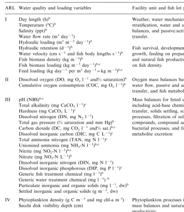
Variables and processes considered by AquaFarm for analysis resolution levels (ARL) I–Va ARL Water quality and loading variables Facility unit and fish lot processes
Day length (h)b Weather, water mechanics and I
Temperature (°C)b stratification, water and salinity mass Salinity (ppt)b balances, and passive/active heat Water flow rate (m3 day−1) transfer.
Hydraulic loading (m3m−2day−1)d
Fish survival, development and Hydraulic retention (d−1)b
growth, feeding on prepared feeds,
II Dissolved oxygen (DO, mg O2l−1and% saturation)b Oxygen mass balances based on water flow, passive and active Cumulative oxygen consumption (COC, mg O2l−1)b
transfer, and fish metabolism.
Mass balances for listed compounds, III pH (NBS)b,c
including acid-base chemistry, gas Total alkalinity (mg CaCO3 l−1)c
Hardness (mg CaCO3L−1)c transfer, solids settling, soil Dissolved nitrogen (DN, mg N2 l−1) processes, filtration of solids and Total gas pressure (% saturation and mm Hg)b compounds, compound addition,
bacterial processes, and fish Carbon dioxide (DC, mg CO2l−1and% sat.)b,c
Dissolved inorganic carbon (DIC, mg C L−1)c metabolite excretion Total ammonia nitrogen (TAN, mg N l−1)c
Unionized ammonia (mg NH3-N l−1)b,c Nitrite (mg NO2-N l−1)b,c
Nitrate (mg NO3-N L−1)b
Dissolved inorganic nitrogen (DIN, mg N l−1) Dissolved inorganic phosphorous (DIP, mg P l−1)c Generic fish treatment chemical (mg l−1)b Generic water treatment chemical (mg l−1)b
Particulate inorganic and organic solids (mg l−1, dw)b Settled inorganic and organic solids (g m−2, dw)
IV Phytoplankton density (g C m−3and mg chl-a m–3) Phytoplankton processes included in mass balances and natural fish Secchi disk visibility depth (cm)
productivity
Total borate (mg B L−1)c
V Mass balances for listed compounds
Total silicate (mg Si L–1)c Total sulfate (mg S L–1)c Total sulfide (mg S L–1)b,c
aVariables and processes considered at each level include those in lower levels. Processes at each level can be individually selected.
bWater quality and loading variables to which fish performance can respond. cCompounds participating in acid-base and precipitation-dissolution chemistry. dHydraulic loading is based on water surface area and flow rate.
Fig. 1. Flowchart of the decision support procedure used by AquaFarm for aquaculture facility design and management planning, including progressive analysis levels and iterative procedures of facility and management specification, simulation, and evaluation.
In conjunction with progressive analysis resolution, a design procedure can be staged by the level of scope and detail used in specifying physical components and management strategies of a given facility. For example, design analyses can start with fish performance, using simplified facilities and a minimum of water quality variables and unit processes. When satisfactory results are achieved at simpler levels, increased levels of complexity for modeling facility performance and man-agement strategies are used. By this approach, the feasibility of rearing a given species and biomass of fish under expected environmental conditions is determined before the specific culture system, resource, and economic requirements necessary to provide this culture environment are developed. Major stages of a typical design procedure are listed below, but this progression is completely user controlled.
1. Production trajectory. Fish development, growth, and feeding schedules for
128 D.H.Ernst et al./Aquacultural Engineering23 (2000) 121 – 179
on initial and target fish states. Environmental quality concerns are limited to water temperature and day length, and unit processes are limited to water flow and heat transfer.
2. Production scale. Required water area and volume requirements for fish rearing units are determined, based on initial and target fish numbers, management methods, and biomass density criteria. Natural fish productivity, if considered, is a function of fish density only.
3. Biomass support. Based on fish feed and metabolic loading, facility water transport and treatment systems are constructed to provide fish rearing units with required water flow rates and water quality. The particular variables and unit processes considered depend on the type of facility. Natural fish productiv-ity, if considered, is a function of fish density and primary productivity. 4. Management schedules. Fish and facility management methods and schedules
are finalized, including operation of culture systems, fish lot handling, and fish number, weight, and feeding schedules.
5. Resource budgets. Resource and enterprise budgets are generated and reviewed.
Table 2
Summary of input specification and output performance data considered by AquaFarm
Input specification data
Possible adjustment of parameters for passive physical, chemical, and biological unit processes and fish performance models
Facility location (or climate data files), optional facility housing and controlled climate, and water quality and capacity of source water(s)
Configuration of facility units for facility water transport, water treatment, and fish culture systems Specifications of individual facility units, including dimensions, elevations and hydraulics, soil and
materials, housing, and water transport and treatment processes
Fish species, fish and facility management strategies, and production objectives (target fish weights/states and numbers at given future dates)
Unit costs for budget items and additional budget items not generated by AquaFarm
Output performance data
Fish number and development schedules for broodfish maturation and egg incubation Fish number, weight, and feed application schedules for fish growout, including optional
consideration of fish weight distributions within a fish lot Fish rearing unit usage and fish lot handling schedules
Tabular and graphical compilations of time-series data for fish performance variables, reported on a fish population and individual fish lot basis, including fish numbers and state, bioenergetic and feeding variables, and biomass loading and water quality variables
Tabular and graphical compilations of time-series data for facility performance variables, reported on a facility and individual facility unit basis, including climate, water quality, fish and feed loading, water flow rates and budgets, compound budgets, process rates, resource use, waste production, and water discharge
Fig. 2. Overview of the software architecture and program components that comprise AquaFarm (see Table 3 for facility unit descriptions). Connecting lines denote communication pathways for method and data access.
4. AquaFarm architecture and components
130 D.H.Ernst et al./Aquacultural Engineering23 (2000) 121 – 179
4.1.User interface and data management
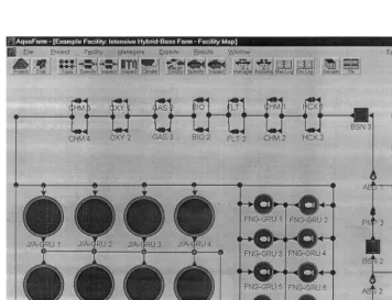
The user interface is typical of window based software, providing a hierarchical menu system and selectable viewing windows that support general-to-specific interface navigation. Types of windows include tool bars, facility maps, specifica-tion sheets, output tables and graphs, management schedules, budget spreadsheets, and user help screens. An example of the interface is shown in Fig. 3 (see recirculation systems under AquaFarm application for additional explanation). According to the type of facility under design and analysis resolution level in use, user access to windows, controls, and data fields is limited to relevant items. Data files are used to store and retrieve user projects, with specification and review mechanisms for data files provided within AquaFarm. Output data can be exported in delimited format for use in computer spreadsheets.
4.2.Domain experts
Domain experts provide expertise in aquaculture science and engineering in the form of quantitative methods and models. These methods consist of property, equilibrium, and rate calculations of physical, chemical, and biological unit pro-cesses and their rules of application. These methods are used to calculate terms in facility-unit and fish-lot state equations and to support management analyses. The documentation required to fully describe these methods is not possible within the size constraints of this paper. Methods of the aquatic chemist, aquacultural engineer, aquatic biologist, and fish biologist are summarized in the appendix, and the enterprise accountant is described below.
4.2.1. Enterprise accountant
The enterprise accountant is responsible for compiling enterprise budgets, which are used to quantify net profit or loss over specified production periods (Meade, 1989; Engle et al., 1997). Enterprise budgets are particularly appropriate for comparing alternative facility designs, in which partial budgets are utilized that focus on cost and revenue items significantly influenced by proposed changes. Additional financial statements (e.g. cash flow and net worth), economic feasibility analyses (e.g. net present value and internal rate of return), and market analyses are required for comprehensive economic analyses (Shang, 1981; Allen et al., 1984; Meade, 1989) but are not supported by AquaFarm.
Cost items (e.g. fish feed) and revenue items (e.g. produced fish) can be specified and budgets can be summarized according to various production bases, time periods, and cost types. Item and budget bases include per unit production area, per unit fish production, and per total facility. Item and budget periods include daily, annual, and user specified periods. Cost types include fixed and variable costs, as determined by their independence or dependence on production output, respec-tively. Fixed costs include items such as management, maintenance, insurance, taxes, interest on owned capital (opportunity costs), interest on borrowed capital, and depreciation for durable assets with finite lifetimes. Variable costs include items such as seasonal labor, energy and materials, equipment repair, and interest on operational capital.
132 D.H.Ernst et al./Aquacultural Engineering23 (2000) 121 – 179
with cost and revenue items totaled and net profit or loss calculated. Net profit values can also be used as net return values to cost items that are not included in
the budget, e.g. net return to land, labor, and/or management.
4.3.Facility site, facility units, and resource units
An aquaculture facility is represented by a facility site, facility units, and resource units. A facility site consists of a given location (latitude, longitude, and altitude), ambient or controlled climate, and configuration of facility units. Facility units consist of water transport units, water treatment units, and fish rearing units (Table 3). Resource units supply energy and material resources to facility units, maintain combined peak and mean usage rates for sizing of resource supplies, and compile total resource quantities for use in enterprise budgets (Table 4). A facility configu-ration is completely user specified and can consist of any combination of facility unit types linked into serial and parallel arrays. A facility is built by selecting (from menu), positioning, and connecting facility units on the facility map. Each type of facility unit is provided with characteristic processes at construction, to which additional processes are added as needed. Facility units are shown to scale, in plan view, color coded by type, and labeled by name. To visualize the progress of simulations, date and time are shown, colors used for water flow routes denote presence of water flow, and fish icons over rearing units denote presence of fish as they are stocked, removed, and moved within the facility.
4.3.1. Facility-unit specifications
Facility unit specifications include housing, dimensions and materials, and ac-tively managed processes of water transport, water treatment, and fish production. The purpose of these specifications is to support facility unit modeling. Individual unit processes and associated specifications can be ignored or included, depending on user design objectives and analysis resolution level. Default facility unit specifi-cations are provided during facility construction, but these variables are highly specific to a particular design project and therefore accessible. Managed (active) processes of water transport, water treatment, and fish production are operated according to the specifications of individual facility units, in addition to manage-ment criteria and protocols assigned to facility managers. Water quality is specified for water sources, including temperature regimes, gas saturation levels, optional carbon dioxide and calcium carbonate equilibria conditions, and constant values for the remaining variables. For soil lined facility units, soils are indirectly specified through given water seepage and compound uptake and release rates.
Facility units can be housed in greenhouses or buildings, with controlled air
temperature, relative humidity, day length, and light intensity (solar shading and/or
artificial lighting). Facility units can be any shape and dimensions, constructed from
soil or materials, and any elevation relative to local soil grade. Top, side, and/or
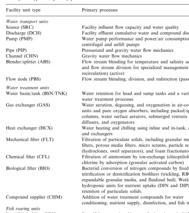
Table 3
Facility unit types and primary processesa
Primary processes Facility unit type
Water transport units
Facility influent flow capacity and water quality Source (SRC)
Discharge (DCH) Facility effluent cumulative water and compound discharge Water pump performance and power/air consumption for Pump (PMP)
centrifugal and airlift pumps
Pressurized and gravity water flow mechanics Pipe (PIP)
Gravity water flow mechanics Channel (CHN)
Blender/splitter (ABS) Flow stream blending for temperature and salinity adjustment and flow stream division for specialized management (e.g. recirculation) (active)
Flow stream blending, division, and redirection (passive) Flow node (PBS)
Water treatment units
Water basin/tank (BSN/TNK) Water retention for head and sump tanks and a variety of water treatment processes
Gas exchanger (GAS) Water aeration, degassing, and oxygenation in air-contact units and pure oxygen absorbers, including packed/spray columns, water surface aerators, submerged venturis and diffusers, and oxygenators
Heat exchanger (HCX) Water heating and chilling using inline and in-tank, elements and exchangers
Mechanical filter (FLT) Filtration of particulate solids, including granular media filters, porous media filters, micro screens, particle separators (hydroclones, swirl separators), and foam fractionators Chemical filter (CFL) Filtration of ammonium by ion-exchange (clinoptilolite) and
chlorine by adsorption (granular activated carbon) Biological filter (BIO) Bacterial conversion of nitrogen compounds by fixed-film
nitrification or denitrification biofilters (trickling, RBC, expandable granular media, and fluidized bed). Wetland and hydroponic units for nutrient uptake (DIN and DIP) and retention of particulate solids.
Compound supplier (CHM) Addition of water treatment compounds for water
conditioning, nutrient supply, disinfection, and fish treatment Fish rearing units
Broodfish maturation: biomass, feed, and metabolic loading Broodfish holding (BRU)
Egg incubator (ERU) Egg incubation: biomass and metabolic loading
Growout rearing (FRY-, FNG-, Fish growout: biomass, feed, and metabolic loading (default types: fry, fingerling, and juvenile/adult)
J/A-GRU)
aNames in parentheses are abbreviations for facility mapping. Processes in addition to primary processes can be considered depending on facility unit type (e.g. inclusion of gas exchangers and compound suppliers in fish rearing units or hydraulic solids removal in a water splitter)
134 D.H.Ernst et al./Aquacultural Engineering23 (2000) 121 – 179
4.3.2. Facility-unit state6ariables
In addition to facility unit specifications, which are fixed variables for a given simulation, facility units are defined by dynamic state variables that vary over the course of a simulation (Table 1). Most of these variables correspond to those typically used. Fish and feed loading variables and cumulative oxygen consumption (Colt and Orwicz, 1991b) are included to support analyses that use these variables as management criteria and for reporting purposes. Alkalinity and pH relationships include consideration of dissolved inorganic carbon (carbon dioxide and
carbon-Table 4
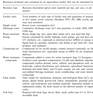
Resources produced and consumed by an aquaculture facility that can be calculated by AquaFarma Resource type Resource description (given units reported per day, per year, or per production
season)
Total numbers of each type of facility unit and quantities of materials used (m2 Facility units
or m3): metal, wood, concrete, fiberglass, PVC, PE, ABS, acrylic, glass, shade tarp, and insulation
Supply water Source water consumption (m3)
Discharge water Cumulative discharge water (m3) and quantities of solids, DIN, DIP, BOD, and COD (kg)
Waste sludge (kg, dw), spent filter media (m3), and dead fish (kg) Waste materials
Energy consumed by facility lighting, water pumps, gas and heat exchangers, Energy
UV sterilizers, etc., expressed as electrical power (kWhr) or energy equivalent of liquid fuels (L; gasoline, methanol, and diesel) or gas fuels (m3; natural gas, propane, and methane)
Compressed air for air-lift pumps, column aerators (optional), air diffusers, and Compressed air
foam fractionators (m3; equivalent energy as kWhr for air compression and delivery)
Water treatment Compounds added to water for water treatment (kg): (1) Inorganic and organic compounds fertilizers (user specified composition), (2) pH and alkalinity adjustment
compounds (carbon dioxide, nitric, sulfuric, and phosphoric acid, sodium hydroxide, sodium bicarbonate and carbonate, agricultural limestone, and hydrated and burnt lime), and (3) pure oxygen, sea salt, and various user-defined fish/egg treatment, water conditioning, and water disinfection compounds
Filter media for mechanical, chemical, and biological filters (m3): sand, expanded Filter media
plastic, plastic beads, gravel/rock, fabric, clinoptilolite, granular activated carbon, and hydroponic and wetland materials. Quantities include original and replacement media, the latter based on the allowed number of regeneration cycles
Prepared fish feeds (kg): larval, flake, mash, pellet sizes 0.5 to 10.0 mm, and Fish feed
broodfish feeds
Stocked and Broodfish, eggs, and growout fish (number, kg) input and output by the facility produced fish
To assist specification of required labor, the enterprise budget provides: (1) per Labor
unit production area and per unit fish production cost bases; (2) total time of fish culture (days); and (3) numbers of management tasks completed for process rate adjustments and fish feeding and handling events
ates) and additional constituents of alkalinity (conjugate bases of dissociated acids). Constituents of dissolved inorganic nitrogen include ammonia, nitrite, and nitrate, and dissolved nitrogen gas can be considered. Dissolved inorganic phosphorous is considered equivalent to soluble reactive phosphorous (orthophosphate) and con-sists of ionization products of orthophosphoric acid (Boyd, 1990). For simplicity, other dissolved forms of phosphorous are not considered and inorganic phospho-rous applied as fertilizer is assumed to hydrolyze to the ortho form based on given fertilizer solubilities. Nitrogen and phosphorous are variable constituents of organic particulate solids, released in dissolved form when these solids are oxidized. Fish and water treatment chemicals are user-defined compounds that may be used for a variety of purposes, such as control of fish pathogens, water disinfectants and compounds present in source waters (e.g. ozone and chlorine), and water condition-ing (e.g. dechlorination). Borate, silicate, and sulfate compounds can have minor impacts on acid-base chemistry, especially for seawater systems, but can normally be ignored.
Particulate solids are comprised of suspended and settleable, inorganic and organic solids (expressed in terms of dry weight, dw; live phytoplankton not included). Suspended inorganic solids (clay turbidity) are considered in order to account for their impact on water clarity (expressed as Secchi disk visibility), which is a function of total particulate solid and phytoplankton concentrations. Settleable
inorganic and organic solids originate from various sources, e.g. in/organic
fertiliz-ers, dead phytoplankton, uneaten feed, and fish fecal material. Settling rates and carbon, nitrogen, and phosphorous contents of these solids depend on their sources. Settled solids originate from combined inorganic and organic settleable solids, and their composition varies in response to their sources.
4.3.3. Facility-unit processes
136
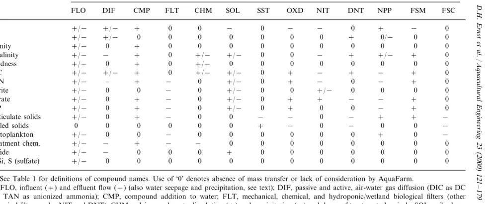
Presence of sources (added:+) and sinks (removed: −) of the listed compounds for the physical, chemical, and biological mass transfer processes occurring in facility unitsa
Facility unit processesb
Compound
FLT CHM SOL SST OXD NIT DNT NPP FSM FSC
DIF
aSee Table 1 for definitions of compound names. Use of ‘0’ denotes absence of mass transfer or lack of consideration by AquaFarm.
bFLO, influent (+) and effluent flow (−) (also water seepage and precipitation, see text); DIF, passive and active, air-water gas diffusion (DIC as DC
In addition to compounds, the water volume contained by a facility unit is subject to mass transfer, including influent and effluent flow, seepage infiltration and loss, precipitation and runoff, and evaporation. Compound transfer via water transfer are based on the assumptions that seepage water constituents are compara-ble to the bulk water volume, precipitation water is pure other than dissolved gases, and evaporation water has no constituents. Settled solids accumulate as a function of contributing particulate solids and settling rates, their lack of disturbance (scouring), and incomplete bacterial oxidation. The accumulation of settled solids can remove significant quantities of nutrients and oxygen demand and provide local anaerobic conditions that support denitrification. Settled solids can be removed by periodic manual procedures (e.g. rearing unit vacuuming and filter cleaning) or continuous hydraulic procedures (e.g. dual-drain effluent configurations).
Facility unit differential equations are based on completely mixed hydraulics (James, 1984a; Tchobanoglous and Schroeder, 1985). While plug-flow hydraulics characterize certain types of facility units, e.g. raceway fish rearing units, the necessity to consider plug-flow hydraulics with respect to overall simulation accu-racy is currently being assessed. When water stratification is considered, a facility unit is modeled as two horizontal water layers of equal depth, and process rates and state variables associated with each layer are maintained separately. Each of these layers is completely mixed internally, and layers inter-mix at a rate dependent on environmental conditions. Possible stratified processes include physical processes (e.g. surface heat and gas transfer), chemical processes (e.g. pond soils), and biological processes (e.g. primary productivity and settled solid oxidation). Possible stratified water quality variables include temperature, dissolved gases, pH and alkalinity, nitrogen and phosphorous compounds, and organic particulate solids. For simplification, phytoplankton are assumed to maintain a homogenous distribu-tion over the water column.
4.3.4. Water transport units
138 D.H.Ernst et al./Aquacultural Engineering23 (2000) 121 – 179
4.3.5. Water treatment units
Water treatment units are used to add, remove, and convert water borne compounds and adjust water temperature (Table 3). Water treatment units typically specialize in a particular unit process, but processes can be combined with a single facility unit as desired. Water treatment processes are primarily defined by their given efficiencies or control levels. Specifications include set-point levels, set-point tolerances, efficiencies of energy and material transfer, minimum and maximum allowed process rates, and process control methods.
Process efficiency is the primary control variable for filtration processes that remove compounds from the water. For mechanical and chemical filters, process efficiency is specified as percent removal of the given compound per pass of water through the filter. For biological filters, process efficiency is specified as kinetic parameters of bacterial processes. For all filters, periodic requirements for media cleaning (removal of accumulated solids) or regeneration (e.g. clinoptilolite and granular activated carbon) over the course of a simulation can be accomplished manually by the facility manager or automatically by the facility unit.
Set-point level is the primary control variable for processes that add compounds to the water and for temperature adjustment, for which the units used to express set-point levels are those of the controlled variable. Pond fertilization is managed
with respect to set points for DIC, DIN, and/or DIP. For each process, constant
rate, simple on/off, and proportional (throttled) process control methods can be
used, the latter providing process rates that vary continuously or in discrete steps over their given operational ranges. Integral-derivative process control can be combined with proportional control so that the rate of change and projected future level of the controlled variable are considered in rate adjustments. Proportional and integral-derivative controls are used to minimize oscillation of the controlled variable around its set-point level (Heisler, 1984). Process control can be accom-plished manually by the facility manager or automatically by the facility unit. For some conditions, for example when both heaters and chillers are present, the controlled variable can be both decreased and increased to achieve a given set point. More typically, controlled variables can only be decreased or increased, for example the addition of a compound to achieve a desired concentration. Set-point tolerances and minimum and maximum allowed process rates are normally required for realistic simulations, for example diurnal control of fish pond aerators in response to dissolved oxygen.
4.3.6. Fish rearing units
Fish rearing units can be designated for particular fish stocks (species), fish life stages (broodfish, eggs, and growout fish), and fish size stages (e.g. fry, fingerling,
and juvenile/adult) (Table 3). This supports movement of fish lots within the facility
4.4.Fish stocks, populations, and lots
Production fish are represented at three levels of organization: fish stocks, fish populations, and fish lots. A fish stock consists of one or more fish populations, and a fish population is divided into one or more fish lots. A fish stock is a fish species or genetically distinct stock of fish, identified by common and scientific names and defined by a set of biological performance parameters. Parameter values are provided for major aquaculture species and can be added for additional aquaculture species. Fish populations provide a level of organization for the management and reporting tasks of related, cohort fish lots. Fish populations are uniquely identified by their origin fish stock, life stage (broodfish, egg, or growout), and production year. Broodfish, egg, and growout fish populations from the same fish stock are linked by life stage transfers, i.e. from broodfish spawning to egg
stocking and from egg hatching to larvae/fry stocking.
Fish lots are fish management units within a fish population. Fish lots are defined by their current location (rearing unit), population size, and development state. The latter consists of accumulated temperature units (ATU) and photoperiod units (APU) for broodfish lots, accumulated temperature units for egg lots, and fish body weights for growout fish lots. At a point in time, fish lot states are maintained as mean values and fish weights within a growout fish lot can be represented as weight distributions (histograms). Variability in fish weights within a growout fish lot can be due to variability present at facility input, fish lot division and combining, and variability in fish growth rates due to competition for limited food resources. Target values for fish lot numbers and states are specified as production objectives or, in the case of broodfish and egg target states, represent biological requirements. Initial values for these variables can be user specified, result from life stage transfers, or result from fish stocking conditions that are required to achieve fish production objectives. Intermediate fish lot numbers and states are predicted by simulation. Methods used to model fish survival, development and growth, feeding, and metabolism are summarized in Appendix A, under the fish biologist domain expert.
4.5.Facility managers
140 D.H.Ernst et al./Aquacultural Engineering23 (2000) 121 – 179
4.5.1. Physical plant manager
Actively managed mass and energy transfer processes of facility units are controlled by the physical plant manager to maintain water quantity and quality variables at desired levels, including water flow, heat and gas transfer, and compound conversion, addition, and removal. Based on facility specifications, active process rates can be adjusted: (1) manually, to emulate manual tasks of the physical plant manager (e.g. manual on-demand aeration); or (2) automatically, to emulate automated process control (e.g. automated on-demand aeration). Manual management tasks are simulated at the management time step, and automated management tasks are simulated at the simulation time step. For aquaculture facilities, water flow rates are based on demands at fish rearing units, as determined by the fish culture manager. For non-aquaculture facilities, water flow rates are controlled at water sources, to give constant or varying water flow rates. Water flow rates can be constrained by source water capacities and by water flow mechanics and hydraulic loading constraints of facility units. Water management schemes include: (1) static water management with loss makeup to maintain minimum volumes; (2) water flow-through with optional serial reuse; and (3) water recircula-tion at specified water recircularecircula-tion and makeup rates.
4.5.2. Fish culture manager — production objecti6es
The fish culture manager is responsible for maintaining fish environmental criteria and satisfying fish production objectives. This is accomplished through the control of water flow and treatment processes, fish feeding rates, and fish biomass management. These tasks are performed according to assigned management respon-sibilities, fish handling and biomass loading management strategies, and available facility resources. Fish production objectives are not achieved if they exceed fish performance capacity or required facility resources are not available.
Fish production objectives are specified as: (1) calendar dates; (2) fish population numbers; and (3) fish development states (broodfish and eggs) or weights (growout fish) at initial fish stocking and target transfer events. Fish transfer events include fish input to the facility, fish life stage transfers within the facility, and fish
release/harvest from the facility. Alternatively, fish stocking specifications can be
determined by AquaFarm such that target objectives are achieved. Production objectives are specified as combined quantities for fish populations and are divided into component values for fish lots. Fish lots within a fish population can be managed in a uniform manner or individually specified for temporal staging of fish production. Fish management size stages can be specified for growout lots to allow assignment of designated rearing units (e.g. fry, fingerling, and on-growing) and types of fish feed (pellet size and composition) based on fish size.
4.5.3. Fish culture manager–en6ironmental criteria
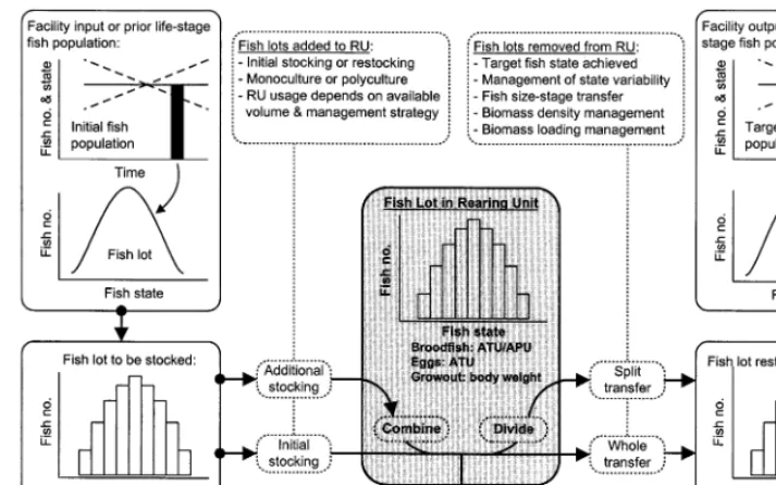
Fig. 4. Management of fish lot stocking, division, combining, and transfer, as based on fish input and output of the facility, life stage transfers within the facility, and fish management strategies. Fish state (see text for definitions) of individual fish lots can be maintained as histograms, normal distributions, or mean values.
carbon dioxide saturation, and concentrations of un-ionized ammonia and
particu-late solids (Table 1). In addition, water temperature, day length, and/or feed
availability can be controlled to achieve desired fish development and growth rates. Management criteria are based on reported biological criteria for the given fish species and allowed deviations beyond designated, optimal biological ranges. Bio-logical criteria are provided and user accessible for major aquaculture species and may be added for additional aquaculture species. For lower analysis resolution levels and systems with known capacities, water exchange rate, fish biomass density
and loading rate, and/or feed loading rate can serve as measures of metabolic
loading. Biomass density management can consider critical density thresholds regarding natural fish productivity and production intensity constraints, in addition to metabolic support considerations. For fish stocking, biomass density constraints are used to allocate fish lots among rearing units.
4.5.4. Fish culture manager–fish lot handling and biomass management
142 D.H.Ernst et al./Aquacultural Engineering23 (2000) 121 – 179
achievement of threshold fish size stages, life stage transfers, and release or harvest target fish states (Fig. 4). Fish handling and biomass management responsibilities are defined by the following options.
1. The use of rearing units is prioritized such that minimum overall fish densities are maintained and either (a) fish lots are never combined or (b) lots are combined only as required to stock all lots. Alternatively, the use of rearing units is prioritized such that maximum overall fish densities are maintained and either (c) lots are combined as required to stock all lots or (d) lots are combined whenever possible to minimize use of rearing units and maximize fish densities.
2. If a facility holds multiple fish stocks, then either (a) different stocks are maintained in separate rearing units (multi-species facilities) or (b) designated stocks are combined within rearing units (polyculture facilities).
3. Fish lots are divided at stocking events to multiple rearing units as required by
fish density constraints (yes/no). During culture, fish lots are transferred to
smaller rearing units if fish densities are too low (yes/no), and/or fish lots are transferred whole or divided to larger rearing units if fish density is too high (yes/no).
4. Based on specified fish biomass loading and water quality criteria, (a) rearing
unit water flow rates are adjusted and/or (b) fish lots are transferred whole or
divided to additional rearing units (adjustment of active process rates of fish rearing units is based directly on given set-point levels).
5. Growout fish lots are graded and divided during culture to reduce excessive
variability in fish weight (yes/no) and/or remove culls (yes/no). Growout fish
lots are high graded and divided at transfer events to leave low grades for further culture (yes/no) and/or remove culls (yes/no).
4.5.5. Fish culture manager–management intensity and risk
4.5.6. Fish culture manager–broodfish maturation and egg incubation
Broodfish maturation is defined by accumulated temperature and/or
photo-period units. Spawning occurs when required levels of these units are achieved, as defined by species-specific parameters maintained by the fish biologist. Water temperature and day length can be controlled to achieve desired maturation rates and spawning dates. Fish population number and spawning calculations account for female-male sex ratios, egg production per female, and fish spawning charac-teristics (i.e. once per year, repeat spawn, or death after spawning).
Egg development is defined by accumulated temperature units. Achievement of development stages (eyed egg, hatched larvae, and first-feeding fry) is based on temperature unit requirements of each stage, as defined by species-specific parameters maintained by the fish biologist. Egg handling can be restricted dur-ing sensitive development stages. Water temperature can be controlled to achieve desired development rates and first-feeding dates.
4.5.7. Fish culture manager — fish growout
Feeding strategies for fish growout can be based on: (1) endogenous (natural) food resources only; (2) natural foods plus supplemental prepared feeds; or (3) prepared feeds only. Natural food resources can be managed indirectly by con-trol of fish densities and maintenance of nutrient levels for primary productivity. Prepared feeds are defined by their proximate composition and pellet size, and specific feed types can be assigned to specific fish size stages. Prepared feeds are applied as necessary to achieve target growth rates, based on initial and target fish weights and dates and considering any contributions from natural foods. For daily simulations, prepared feed is applied once per day. For diurnal simulations, feed is applied according to the specified number of feedings per day and length of the daily feeding period, which can be specific to fish size stage. In addition, the impact of feed allocation strategies and application rates on food conversion efficiency and fish growth variability due to competition for limited food re-sources can be considered.
5. Facility and management simulation
5.1.Simulation processing
144 D.H.Ernst et al./Aquacultural Engineering23 (2000) 121 – 179
steps; and (3) for purposes of numerical integration, maintains arrays of state variables and finite difference terms for the differential equations of facility units and fish lots. The simulation manager processes simulation objects in a generic manner and has no need to be concerned with specific details of individual objects, e.g. differential equations used to calculate difference terms or the man-agement protocols used by facility managers.
Manual procedures of the physical plant and fish culture managers are discon-tinuous, discrete events. Managers respond to update commands over a series of management time steps by reviewing their assigned responsibilities, responding as facility resources allow, and logging management problems and completed tasks to management logs. In contrast, facility units and fish lots consist of continuous processes, represented by sets of simultaneous differential equations. Facility units and fish lots are simulated by solving state equations, updating state variables, and logging state variable and process rate data over a series of simulation time steps. The state variables and equations used for facility units and fish lots depend on the analysis resolution level, fish performance methods, and passive and active unit processes under consideration. At each simulation step, domain experts are used to calculate property, equilibrium, and process rate terms used in differential equations and management tasks.
5.2.Deterministic simulation
5.3.Numerical integration
Facility unit and fish lot differential equations can be solved by numerical or analytical methods. Under numerical integration, differential equations are used as finite difference equations to calculate finite difference terms (unit mass or energy per time). Related simulation objects are processed as a group, as determined by the existence of shared variables and simultaneous processes. State variables and finite difference terms of related simulation objects are collected into arrays at each simulation step and solved by the simulation manager using simultaneous, fourth-order Runge – Kutta integration (RK4; Elliot, 1984). RK4 integration is a powerful numerical integration method, capable of solving complex sets of simultaneous differential equations. However, RK4 integration may require small time steps, on the order of minutes to hours, when high rates of energy or mass transfer characterized by first-order kinetics exist in facility units (e.g. high rates of water flow, active gas transfer, or fixed-film bacterial processes). In addition, RK4 integration requires four iterations per time step for the calculation of difference terms and update of state variables. Together, these requirements may result in excessively long simulation execution times (e.g. 3 min, real time), depending on the number of simulation objects, length of the simulation period, and computer processing capacity.
5.4.Analytical integration
Analytical integration methods can accommodate high rate, first-order processes at large time steps (e.g. 1 day) and can be used to minimize required calculations and simulation execution times. However, aquaculture facilities are typically char-acterized by simultaneous processes within and among facility units, and achieve-ment of analytical solutions normally requires the use of simplifying assumptions. To explore tradeoffs between mathematical rigor and simulation processing times, combined numerical-analytical and simplified analytical integration methods were developed. For combined numerical-analytical integration, difference terms for each of the four cycles of RK4 integration are calculated using analytical integration. For simplified analytical integration, differential equations are simplified to a level where analytical solutions can be attained (Elliot, 1984). By this simplification, some simultaneous processes are unlinked, and thus simulation objects and the variables they contain are updated in order of their increasing dependence on other objects and variables. The simulation order used is facility climate, up to down stream facility units, and finally fish lots. In addition, variables within a facility unit are updated in order of increasing dependence on other variables, beginning with water temperature.
5.5.Management and simulation time steps
146 D.H.Ernst et al./Aquacultural Engineering23 (2000) 121 – 179
fish culture managers. The size of the simulation time step is based on the nature of the aquaculture system and temporal resolution required to adequately capture system dynamics. Daily simulations (e.g. 1-day time step), for which diurnal variables and processes are expressed and used as daily means, always represent some level of simplification at a degree depending on the type of facility and analysis resolution level. For example, all fish culture systems are at least character-ized by diurnal fish process, resulting from day-versus-night activity levels and feeding rates of fish. However, diurnal simulations (e.g. 1-h time step) are required only when the variability of process rates and state variables within a day period, and associated management responses, must be considered to adequately represent the system. For example, diurnal simulations may be used for solar-algae ponds for high-resolution modeling of heat transfer and primary productivity, and they may be used for intensive systems for high-resolution modeling of fish feeding and metabolism. Any consideration of process management within a 24-h period requires diurnal simulations, e.g. pre-dawn aeration for pond-based systems or diurnal control of oxygen injection rates for intensive systems. For RK4 integra-tion, daily simulations may require time steps of less than one day, but variables and processes are still used as daily means.
6. AquaFarm testing, calibration, and validation
The program code modules comprising AquaFarm were tested, debugged, and verified to perform according to the previously reported or newly developed methods from which they were developed. Testing alone was sufficient to validate data input and output, management, and display tasks, integration procedures for differential equations, and simulation of facility management. Similarly, the validity of actively managed processes was largely dependent on given process specifications (e.g. water treatment efficiencies) and confirmed by direct testing. Finally, Aqua-Farm was verified to provide full ranges of expected results (dependent variables) for all types of extensive and intensive aquaculture systems, solely by adjustment of input parameters and independent variables over their reasonable ranges. In sum, this testing verified the internal and external consistency of AquaFarm (Cuenco, 1989) and indicated sufficient development of the collected parameters, variables, and unit processes considered and their combined expression as differential equa-tions and integrated funcequa-tions.
are given in Appendix A. For some component models, these accomplishments are
preliminary and/or rely on parameter values from the supporting literature.
Com-pletion of calibration and validation procedures for selected, unit process models is ongoing, as described in the conclusion to this paper.
7. AquaFarm application
Application of AquaFarm to various aquaculture systems and analyses is demon-strated in the following examples. For each exercise, site-specific facility variables, management strategies, and model parameters were entered into AquaFarm. Addi-tional parameters of unit process models were based on default values provided by AquaFarm. Simulations were then performed to generate fish culture schedules, chronologies of facility state variables and processes, and required resources to achieve fish production objectives. Finally, predicted performance data were com-pared to empirical data from representative studies in the literature.
Reporting of the specifications and results of these simulation exercises is limited to overviews, with a focus on core issues of fish performance and dominant facility processes. The specifications and results presented are not necessarily meant to represent critical variables, but rather to illustrate the range of detail and analytical capacities available in AquaFarm. The design procedure presented earlier is not demonstrated, rather the results of a single simulation are presented for each system type. Enterprise budgets are not presented, for which unit costs are highly specific to location and budget formats have already been described. While not shown, however, any of these examples could use a series of simulations to consider resource use, management intensity, and budgetary requirements over a range of fish production levels and alternative design and management strategies.
For all of these exercises, it is emphasized that the accuracy of simulation results relative to empirically determined results was highly dependent on the accuracy of site-specific variables and parameters. When simulation results are said to be ‘comparable’ to the referenced studies, it is meant that simulation results were within the range of reported results and showed similar cause-and-effect behavior for independent and dependent variables. Conclusions for these exercises include the caveat that fully comprehensive reporting of methods and results were not available in the studies used, as is typical in technical papers, requiring the estimation of some design and management variables.
148 D.H.Ernst et al./Aquacultural Engineering23 (2000) 121 – 179
7.1.Tilapia production in ponds
AquaFarm was applied to the production of Nile tilapia (Oreochromis niloticus)
in tropical (10° latitude) solar-algae ponds. Specifications and results of this exercise are provided in Table 6 and Figs, 5, 6, and 7. Diurnal simulations were used and water stratification was considered. Agriculture limestone (calcium carbonate) and fertilizer were applied to maintain DIC (in terms of alkalinity), DIN, and DIP nutrient levels for primary productivity. Fertilized ponds received lime and fertilizer only. Fertilized-fed ponds received lime and fertilizer by the same management criteria as fertilized ponds, with additional application of pelletized feed as required to achieve target fish growth rates. Fertilizer consisted of combined chicken manure and ammonium nitrate, with the latter added to achieve a nitrogen-phosphorous ratio of 5.0, based on the manure nitrogen and phosphorous contents (Lin et al., 1997). Predicted water quality regimes and fertilizer and feed requirements were com-parable to reported values for tilapia production under similar site and management conditions. As expected, total lime application rates were in the low range of reported rates (Boyd, 1990; Boyd and Bowman, 1997), for which pond source water had low alkalinity but soils were assumed to already be neutralized with respect to exchange acidity (base unsaturation). The nitrogen and phosphorous application rates used were within reported ranges for tilapia production in fertilized ponds, which range
2.0 – 4.0 kg N ha−1day−1 at N:P ratios that range 1:1 – 8:1 (Lin et al., 1997). For
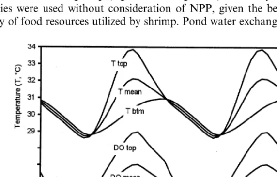
fertilized and fertilized-fed ponds, simulated fish growth rates and total production per hectare, fish density level at the onset of feeding, and required feed application rates were comparable to reported results (Diana et al., 1996; Diana, 1997; Lin et al., 1997). Fish production and application of fertilizer and feed were adequately estimated using a daily time step with no consideration of water stratification. However, as generally found for solar-algae ponds, diurnal simulations and con-sideration of stratification were required to estimate extremes in water quality regimes. Typical diurnal profiles of temperature and dissolved oxygen, as shown in Fig. 7 for mid summer, were comparable to reported profiles for stratified tropical ponds (Losordo and Piedrahita, 1991; Piedrahita et al., 1993; Culberson and Piedrahita, 1994). The maximum divergence in water quality between the top and bottom layers was controlled by the specified regime of daily-minimum layer mixing rates.
7.2.Catfish production in ponds
AquaFarm was applied to production of channel catfish (Ictaluras punctatus) in
temperate (30° latitude) solar-algae ponds. Specifications and results of this exercise are provided in Table 7 and Figs. 8, 9, and 10. Diurnal simulations were used and water stratification was considered. Single fish stocking and harvest events were used to simplify this example, rather than the periodic high-grade harvesting and partial re-stocking methods typically employed for catfish production. Target fish numbers and weights were specified such that feed application rate increased to a maximum
Table 6
Example application: tilapia production in fertilized and fed ponds
Specifications
Facility Location: 10 N latitude; 10 m elevation
Weather: annual regimes for air temperature, cloud cover, precipitation, and water mixing index (stratification)
Source water quality: 20 mg l−1 alkalinity and equilibrium gas concentrations
Levee type, clay lined ponds, 1.0 ha in area, and 1.0 m average depth Culture systems
Water makeup to replace losses and maintain depth
Pond unit processes used: water budget, passive heat transfer, seasonal water stratification, passive gas transfer, solids settling, primary productivity, bacterial processes (organic oxidation, nitrification, and denitrification), soil processes, and fish processes
Fertilizer composition: chicken manure with ammonium nitrate added to achieve an N:P ratio of 5.0, with a combined composition of 22.4% N, 4.48% P, and 70% dry wt. organic solids
Feed composition: 35% protein, 1.5% phosphorous
Fertilized ponds (see Table 1 for units): agricultural limestone and mixed inorganic/organic fertilizer applied to maintain DIC (alkalinity\6 40), DIN (\6 1.0), and DIP (\6 0.1), beginning 6 weeks prior to fish stocking Fertilized-fed ponds: additional application of prepared feed as required to achieve target fish growth rates
Culture period: March 1 to Oct. 1 (215 days) Fish production
objectives
Fish number: 10 000–9000 fish ha−1at 10% mortality
Fish weight: 1.0 g at stocking to weight available on Oct. 1 for fertilized ponds, and 1.0–512 g target weight for fertilized-fed ponds
Results
Fertilized pond applications: total lime applied 1870 kg ha−1, fertilizer Fish production
applied at a mean rate of 12.3 kg ha−1d−1(2.8 kg N ha−1day−1and 0.55 kg P ha−1day−1) over the pond pre-conditioning and fish rearing period Fertilized-fed pond applications: total lime applied 1900 kg ha−1, fertilizer requirements reduced about 10%, supplemental feed applied at an increasing rate to a maximum of 65 kg ha−1day−1over a 70-day end period Fertilized pond production: 332 g fish at 3000 kg fish ha−1on Oct. 1 Fertilized-fed pond production: 512 g fish at 4600 kg fish ha−1on Oct. 1, 80% fish feeding index (% maximum ration) to achieve target weight, and 170% food conversion efficiency (based on applied feed only, mortality included)
150 D.H.Ernst et al./Aquacultural Engineering23 (2000) 121 – 179
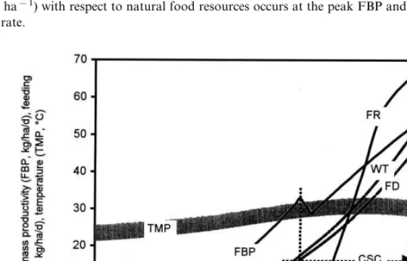
Fig. 5. Simulated data (1-h time step) for tilapia production in fertilized ponds over a 7-month culture period. The temperature band represents the diurnal temperature regime. Critical standing crop (CSC, 1600 kg ha−1) with respect to natural food resources occurs at the peak FBP and inflection point of fish growth rate.
Fig. 6. Simulated data (1-h time step) for tilapia production in fertilized and fed ponds over a 7-month culture period. The temperature band represents the diurnal temperature regime. Critical standing crop (CSC, 1600 kg ha−1) with respect to natural food resources is achieved, followed by a short decline in FBP until the onset of supplemental feeding.
production period, from June 1 year 1 to October 31 year 2 (519 days), included a fish over-wintering period.
Feed application rates increased over the rearing period in association with increasing fish biomass density as well as varying with water temperature. Fish feeding and growth rates were within typical ranges (Tucker, 1985). Predicted water quality regimes and aeration requirements were comparable to reported values for catfish production, including aeration timing, maximum power requirement, and cumulative power use (Cole and Boyd, 1986; Brune and Drapcho, 1991; Tucker and van der Ploeg, 1993; Schwartz and Boyd, 1994). To match reported aeration requirements (Cole and Boyd, 1986), accurate specifications were required for aerator size, standard aerator efficiency, and minimum allowed dissolved oxygen levels.
7.3.Shrimp production in ponds
AquaFarm was applied to semi-intensive production of marine (penaeid) shrimp in tropical (10° latitude), fertilized, fed, and aerated solar-algae ponds. Results of this exercise (not shown) compared well to marine shrimp production studies (Fast and Lester, 1992; Wyban, 1992; Briggs and Funge-Smith, 1994), including shrimp growth, aeration requirements, and water quality regimes. For estimating natural food resources and timing the initiation of prepared feed application, empirically
based critical standing crop (e.g. 100 – 300 kg ha−1) and carrying capacity shrimp
densities were used without consideration of NPP, given the benthic location and variety of food resources utilized by shrimp. Pond water exchange rates of 0.0 – 30%
152 D.H.Ernst et al./Aquacultural Engineering23 (2000) 121 – 179
Table 7
Example application: channel catfish production in ponds
Specifications
Location: 32 N latitude, 100 m elevation Facility
Weather: annual regimes for air temperature, cloud cover, precipitation, and water mixing index (stratification)
Source water quality: 100 mg l−1alkalinity and equilibrium gas concentrations Culture Levee type, clay lined ponds, 5.0 ha in area, and 1.0 m average depth
Water makeup to replace losses and maintain depth systems
Pond unit processes used: water budget, passive heat transfer, seasonal water stratification, passive and active gas transfer, solids settling, primary productivity, bacterial processes (organic oxidation, nitrification, and denitrification), soil processes, and fish processes
Aeration: on atB30% and off at \6 40% DO saturation based on water quality of bottom water layer, maximum aeration rate 6.25 kW ha−1, and aerator SAE 1.2 kg O2kWhr−1
Fish Culture period: June 1, year 1 to Oct. 31, year 2 (518 days) production Fish number: 12 000 to 10 500 fish ha−1 at 12.5% mortality
Fish weight: 1.0 g at stocking to 880 g target weight objectives
Results
80% fish feeding index (% maximum ration) Fish
production 50% food conversion efficiency
9250 kg ha−1maximum fish biomass density 110 kg ha−1day−1maximum feed application rate
Aeration power use: total of 4260 kWhr ha−1, for 672 total hours of operation, ranging from 2 to 7 h per day, over a period of 4 months
Water quality (see Fig. 8 and Fig. 9): DIN averaged 72% TAN and 28% nitrate, alkalinity 80–100 mg l−1, and diurnal NPP−0.4–5.0 g C m−3day−1(whole column)
per day were simulated and compared, including impacts on pond water quality, tradeoffs in relation to aeration requirements, and compound and BOD loading rates on receiving waters.
thermal stratification, and it is present in aerated/mixed ponds where thermal stratification is broken down. Therefore, it was accounted for by the minimum dissolved oxygen criterion used for aeration management. By increasing this
Fig. 8. Simulated data (1-h time step) for catfish production in fed ponds, showing the last 7 months of the 17 month culture period. Bands for water quality variables represent diurnal, stratified regimes, and top and bottom layers of the water column are shown for temperature and dissolved oxygen. Bottom bands overlay top bands to a large degree and daily water-column turnover is occurring.