Artech House Distortion In RF Power Amplifiers Feb 2003 ISBN 1580535399 pdf

(1)

(2)

(3)

(4)

(5)

Distortion in RF Power Amplifiers

Joel Vuolevi

Timo Rahkonen

(6)

Distortion in RF power amplifiers / Joel Vuolevi, Timo Rahkonen. p. cm. — (Artech House microwave library)

Includes bibliographical references and index. ISBN 1-58053-539-9 (alk. paper)

1. Power amplifiers. 2. Amplifiers, Radio frequency. 3. Electric distortion—Prevention. I. Rahkonen, Timo. II. Title. III. Series.

TK7871.58.P6V79 2003 621.384'12—dc21

2002043669

British Library Cataloguing in Publication Data Vuolevi, Joel

Distortion in RF power amplifiers. — (Artech House microwave library)

1. Power amplifiers 2. Amplifiers, Radio frequency 3. Radio— Interference

I. Title II. Rahkonen, Timo 621.3'8412

ISBN 1-58053-539-9 Cover design by Gary Ragaglia

© 2003 ARTECH HOUSE, INC. 685 Canton Street

Norwood, MA 02062

All rights reserved. Printed and bound in the United States of America. No part of this book may be reproduced or utilized in any form or by any means, electronic or mechanical, in-cluding photocopying, recording, or by any information storage and retrieval system, with-out permission in writing from the publisher.

All terms mentioned in this book that are known to be trademarks or service marks have been appropriately capitalized. Artech House cannot attest to the accuracy of this informa-tion. Use of a term in this book should not be regarded as affecting the validity of any trade-mark or service trade-mark.

(7)

v

Chapter 3 Memory Effects in RF Power Amplifiers

43

3.1 Efficiency ... 43

3.2 Linearization ... 45

3.2.1 Linearization and Efficiency ... 45

3.2.2 Linearization Techniques ... 46

3.2.3 Linearization and Memory Effects ... 48

3.3 Electrical Memory Effects ... 51

3.4 Electrothermal Memory Effects ... 56

3.5 Amplitude Domain Effects ... 59

3.5.1 Fifth-Order Analysis Without Memory Effects 60 3.5.2 Fifth-Order Analysis with Memory Effects ... 62

3.6 Summary ... 66

References ... 68

Chapter 4 The Volterra Model

71

4.1 Nonlinear Modeling ... 71

4.1.1 Nonlinear Simulation Models... 72

4.1.2 The Properties of the Volterra Models ... 75

4.2 Nonlinear I-V and Q-V Characteristics ... 77

4.2.1 I_C-V_BE-V_CE Characteristic... 78

4.2.2 g_pi andr_bb... 82

4.2.3 Capacitance Models ... 82

4.3 Model of a Common-Emitter BJT/HBT Amplifier ... 84

4.3.1 Linear Analysis ... 84

4.3.2 Nonlinear Analysis... 87

4.4 IM3 in a BJT CE Amplifier ... 95

4.4.1 BJT as a Cascade of Two Nonlinear Blocks ... 95

4.4.2 Detailed BJT Analysis... 102

4.5 MESFET Model and Analysis ... 109

4.6 Summary ... 115

(9)

Contents vii

Chapter 5 Characterization of Volterra Models

123

5.1 Fitting Polynomial Models ... 124

5.1.1 Exact and LMSE Fitting... 124

5.1.2 Effects of Fitting Range ... 126

5.2 Self-Heating Effects ... 127

5.2.1 Pulsed Measurements ... 129

5.2.2 Thermal Operating Point ... 131

5.3 DC I-V Characterization ... 133

5.3.1 Pulsed DC Measurement Setup ... 133

5.3.2 Fitting I-V Measurements ... 134

5.4 AC Characterization Flow ... 136

5.5 PulsedS-Parameter Measurements ... 137

5.5.1 Test Setup ... 137

5.5.2 Calibration ... 139

5.6 De-embedding the Effects of the Package ... 140

5.6.1 Full 4-Port De-embedding... 141

5.6.2 De-embedding Plain Bonding Wires ... 143

5.7 Calculation of Small-Signal Parameters ... 145

5.8 Fitting the AC Measurements ... 147

5.8.1 Fitting of Nonlinear Capacitances ... 147

5.8.2 Fitting of Drain Current Nonlinearities ... 149

5.9 Nonlinear Model of a 1-W BJT ... 152

5.10 Nonlinear Model of a 1-W MESFET ... 155

5.11 Nonlinear Model of a 30-W LDMOS ... 160

5.12 Summary ... 165

References ... 167

Chapter 6 Simulating and Measuring Memory Effects

171

6.1 Simulating Memory Effects ... 172

6.1.1 Normalization of IM3 Components ... 172

6.1.2 Simulation of Normalized IM3 Components .. 175

6.2 Measuring the Memory Effects ... 180

6.2.1 Test Setup and Calibration ... 181

6.2.2 Measurement Accuracy ... 184

6.2.3 Memory Effects in a BJT PA ... 185

6.2.4 Memory Effects in an MESFET PA ... 187

6.3 Memory Effects and Linearization ... 187

(10)

References ... 192

Chapter 7 Cancellation of Memory Effects

193

7.1 Envelope Filtering ... 194

7.2 Impedance Optimization ... 198

7.2.1 Active Load Principle ... 199

7.2.2 Test Setup and Its Calibration ... 202

7.2.3 Optimum Z_BB at the Envelope Frequency Without Predistortion ... 203

7.2.4 Optimum Z_BB at the Envelope Frequency with Predistortion ... 204

7.3 Envelope Injection ... 207

7.3.1 Cancellation of Memory Effects in a CE BJT Amplifier ... 209

7.3.2 Cancellation of Memory Effects in a CS MESFET Amplifier ... 211

7.4 Summary ... 217

References ... 220

Appendix A: Basics of Volterra Analysis

221

Reference ... 225

Appendix B: Truncation Error

227

Appendix C: IM3 Equations for Cascaded Second-Degree

Nonlinearities

231

Appendix D: About the Measurement Setups

245

Reference ... 247

Glossary

249

About the Authors

253

(11)

ix

Acknowledgments

Many persons and organizations deserve warm thanks for making this book a reality. To mention a few, Jani Manninen has made many of the measurements and test setups presented in this book, Janne Aikio contributed much to the characterization measurement techniques, and Antti Heiskanen contributed to the higher order Volterra analysis. Mike Faulkner and Lars Sundström originally introduced us to this linearization business. Veikko Porra and Jens Vidkjaer pointed out several important topics to probe further. The grammar and style of this book and the original publications on which it is mostly based have been checked by Janne Rissanen, Malcolm Hicks, and Rauno Varonen. Also, David Choi spent a lot of time with the text to make it more readable and fluent.

The financial and technical support of TEKES (National Technology Agency of Finland), Nokia Networks, Nokia Mobile Phones, Elektrobit Ltd, and Esju Ltd is gratefully acknowledged. The work has also been supported by the Graduate School in Electronics, Telecommunications and Automation (GETA) and the following foundations: Nokia Foundation, Tauno Tönningin säätiö, and Tekniikan edistämissäätiö.

(12)

(13)

1

Chapter 1

Introduction

1.1 Motivation

This book is about nonlinear distortion in radio frequency (RF) power amplifiers (PAs). The purpose of the PA is to boost the radio signal to a sufficient power level for transmission through the air interface from the transmitter to the receiver. This may sound simple, but it involves solving several contradicting requirements, the most important of which are linearity and efficiency. Unfortunately, these requirements tend to be mutually exclusive, so that any improvement in linearity is usually achieved at the expense of efficiency, and vice versa.

To avoid interfering with other transmissions, the transmission must stay within its own radio channel. If the modulated carrier has amplitude variations, any nonlinearity in the amplifier causes spreading of the transmitted spectrum (so-called spectral regrowth). This effect can be reduced by using constant-envelope modulation techniques that unfortunately have quite low data rate/bandwidth ratio. When using more efficient digital modulation techniques, the only solution is to design the amplifiers linear enough.

(14)

1.2 Historical Perspective

In first-generation systems, such as the Nordic Mobile Telephone (NMT) or Advanced Mobile Phone Service (AMPS), the RF signal was frequency modulated (FM). Highly efficient PAs are possible in FM systems because of the fact that no information is encoded in the amplitude component of the signal. Even so, the PA of a mobile phone consumed as much as 85% of the total system power at the maximum power level, thus limiting the on-time of the terminal.

Unlike wired line communications, wireless systems must share a common transmission medium. The available spectrum is therefore limited, and so channel capacity (i.e., the amount of information that can be carried per unit bandwidth) is directly associated with profit. The demand for greater spectral efficiency was addressed by the development of second-generation systems, where digital transmission and time domain multiple access (TDMA) is used, where multiple users are time multiplexed on the same channel. For example, in the Global System for Mobile Communications (GSM), eight calls alternate on the same frequency channel, resulting in cost-effective base stations. The GSM modulation scheme retains constant envelope RF signals, but the need for smooth power ramp up and ramp down of the allocated time-slot transmissions imposes some moderate linearity requirements. This reduces the efficiency of the amplifier, but it is compensated by the fact that the PA in the mobile node is only active one-eighth of the time. This, together with the smart idling modes, allows GSM handsets to achieve very long operating times.

The data transmission capacity of GSM is rather modest, so the obvious solution to increase the achievable bit rate was, as implemented in GSM-EDGE, to use several time slots for a single transmission and to replace the Gaussian minimum shift key (GMSK) modulation scheme with a spectrally more efficient 8-PSK that unfortunately has a varying envelope. So as wireless communication systems migrate towards higher channel capacity, more linear and, consequently, less efficient PAs have become the norm.

(15)

Introduction 3

the mobile transmits on a continuous time basis. Designing an economical PA for these requirements is an enormous engineering challenge.

The situation is not easier in the base stations, either, where the linearity requirements are tighter than in handsets. The trend is towards multicarrier transmitters where a single amplifier handles several carriers simultaneously, in which case the bandwidth, power level, and the peak power to average power ratio (crest factor) all increase. The efficiency of these kinds of power amplifiers is very low, and due to higher total transmitted power, this results in very high power dissipation and serious cooling problems.

1.3 Linearization and Memory Effects

The goal of this book is to improve the conceptual understanding needed in the development of PAs that offer sufficient linearity for wideband, spectrally efficient systems while still maintaining reasonably high efficiency. As already noted, efficiency and linearity are mutually exclusive specifications in traditional power amplifier design. Therefore, if the goal is to achieve good linearity with reasonable efficiency, some type of linearization technique has to be employed. The main goal of linearization is to apply external linearization to a reasonably efficient but nonlinear PA so that the combination of the linearizer and PA satisfy the linearity specification. In principle, this may seem simple enough, but several higher order effects seriously limit its effectiveness, in practice.

Several linearization techniques exist, and they are reviewed in Chapter 3; a much more detailed discussion can be found from [1-3]. Stated briefly, linearization can be thought of as a cancellation of distortion components, and especially as a cancellation of third-order intermodulation (IM3) distortion, and where the achieved performance is proportional to the accuracy of the canceling signals. Unfortunately, the IM3 components generated by the power amplifier are not constant but vary as a function of many input conditions, such as amplitude and signal bandwidth. Here, these bandwidth-dependent phenomena are calledmemory effects.

(16)

techniques are used to cancel out the intermodulation sidebands; in fact, the reported performance of some simple techniques may actually be limited not by the linearization technique itself, but by the properties of the amplifier – and especially by memory effects.

Different linearization techniques have different sensitivities to memory effects. Feedback and feedforward systems (see Section 3.2.2) are less sensitive to memory effects because they measure the actual output distortion, including the memory effects. However, predictive systems like predistortion and envelope elimination and restoration (EER) are vulnerable to any changes in the behavior of the amplifier, and memory effects may cause severe degradation in the performance of the linearizer.

However, there is no fundamental reason why predictive linearization techniques should be poorer than feedback or feedforward systems since the behavior of spectral components, though quite difficult to predict under varying signal conditions, is certainly deterministic. Thus, in theory, real time adaptation or feedback/feedforward loops are not strictly necessary, provided that the behavior of distortion components is known or can be controlled. The primary motivation of this book is to develop a power amplifier design methodology which yields PA designs that are more easily linearized. The approach taken here proposes that, by negating the relevant memory effects, the performance of simple linearization techniques that otherwise do not give sufficient linearization performance, can be significantly improved.

To achieve a significant linearity improvement by means of simple and low power linearization techniques requires detailed understanding of the behavior and origins of the relevant distortion components. This is a key theme that is carried on throughout this book. The actual linearization techniques themselves will not be discussed in detail, but instead, the fundamental aim of this book is to give the designer the crucial insights required to understand the origins of memory effects, as well as the tools to keep memory effects under control.

1.4Main Contents of the Book

(17)

Introduction 5

sufficient for analyzing canceling linearization systems, where subdecibel accuracy is a prerequisite.

In laboratory measurements, the commonly used single-tone amplitude and phase distortion (AM-AM and AM-PM) characterization techniques actually have a zero bandwidth, and so they completely fail to capture bandwidth-dependent phenomena. Therefore, the accuracy of IM3 values resulting from AM-AM and AM-PM models suffers when attempting to model an amplifier that has memory effects. In addition, the AM-AM measurements also suffer from self-heating: The AM-AM measurements are performed using continuous wave (CW) signals, resulting in transistor junction temperatures quite different from those generated in practice, where modulated signals are applied to the PA.

This book presents several techniques that help understand, simulate, measure, and cancel memory effects. The subsequent chapters will provide a detailed discussion of the following topics:

1. A comparison between data available from AM-AM and AM-PM versus IM measurements. Normal single-tone AM-AM measurement has zero bandwidth, but it can be performed using a two-tone signal with variable tone spacing, as well. In this case, the same information about the nonlinearity of the device should be available in both the fundamental and IM3 tones, but the discussion will show that the large fundamental signal masks a considerable amount of fine variations in distortion in AM-AM measurements.

2. To study the phase variations of the IM3 tones, a three-tone measurement system will be presented.

3. Device modeling. Input-output behavioral models can be generated on the basis of a completed amplifier, but these do not yield any information to aid in design optimization. Instead, the analysis presented in this book models the transistor by replacing every nonlinear circuit element (input capacitance,g_m, and so forth) by the parallel combination of a linear circuit element (small-signal capacitance, small-signal g_m, and so forth) and a nonlinear current source. This leads to two important findings:

(18)

b. Distortion is originally generated in form of current, which is converted to a voltage by terminal impedances. Thus, the phase and amplitude of the distortion components can be strongly influenced by the terminal impedances, and especially by the impedances of the biasing networks.

4. Based on the reasoning above, this book includes a review of a distortion analysis technique called Volterra analysis, which is based on placing polynomial distortion sources in parallel with linear circuit elements. The main benefits of this technique are:

a. The dominant sources of distortion can be pinpointed;

b. Phase relationships between distortion contributions can be easily visualized;

c. A polynomial model can be accurately fitted to the measured data; d. The polynomial models can also be used in harmonic balance

simulators.

5. This book also introduces some circuit techniques for reducing memory effects in power amplifiers. The standard method of minimizing memory effects involves attempting to maintain impedances at a constant level over all frequency bands. Unfortunately, other design requirements often interfere with this aim and cause memory effects. To address this problem, an active impedance synthesis technique is introduced, which can be used to drive impedances to their optimum values. What is more, this technique can be used for electrical and thermal memory effects.

6. Finally, the book presents a characterization technique for polynomial nonlinearities. Since many existing power transistor models are not sufficiently accurate in terms of distortion simulations, characterization measurements are the only way of obtaining this information. This is accomplished using pulsed S-parameter measurements over a range of terminal voltages and temperatures.

1.5 Outline of the Book

(19)

Introduction 7

memory, it is important to define nonlinearity, bandwidth dependency, and memory, and to examine their associated effects. Chapter 2 also introduces a direct calculation method for deriving equations for the spectral components generated in such circuits. Due to its analytical nature, this method, based on the Volterra series, provides detailed information about distortion mechanisms in nonlinear systems. Later chapters of this book will describe the use of the method.

Chapter 3 first discusses memory effects from the linearization point of view. Some of the most common linearization techniques are presented, and then the chapter highlights the harmful memory effects in more detail, with a particular focus on electrical and thermal memory effects. Electrical memory effects are those caused by varying node impedances within a frequency band, while thermal memory effects are caused by dynamic variations in chip temperature. Both kinds of memory effects are analyzed by comparing a memoryless polynomial model with measurements of real power amplifier devices. Memory effects tend to be considered merely in terms of modulation frequency, but Chapter 3 also introduces mechanisms that produce memory effects as a function of signal amplitude. These mechanisms are referred to as amplitude domain memory effects.

Chapter 4 discusses transistor/amplifier models and introduces problems related to PA modeling. The amplifier models are classified as either behavioral or device-level models, which are based on some pre-defined, physically based functions or simply on empirical fitting functions. The Volterra model is an empirical model that is capable of providing component-level information that can be used for design optimization. The chapter also gives a derivation of the Volterra models for a common-emitter (CE) bipolar junction transistor (BJT) amplifier and a common-source (CS) metal-semiconductor field effect transistor (MESFET) amplifier. The models take into account the effects of modulation frequency, and temperature, and are therefore able to model memory effects. Moreover, IM products are presented as vector sums of each degree of nonlinearity, thereby providing insight into the composition of distortion, which is instrumental in design optimization.

Chapter 5 discusses the characterization of the Volterra model. The dc characterization is briefly discussed for the sake of clarity, before shifting the focus on a new technique based on a set of small-signal S-parameters measured over a range of bias voltages and temperatures.

(20)

important improvement over measurements based merely on the fundamental signal or amplitude.

Chapter 7 introduces three techniques for canceling memory effects: impedance optimization, envelope filtering, and envelope injection. In addition, the chapter presents the source pull test setup for investigating the effects of out-of-band impedances. Then, a comparison is presented between envelope filtering and envelope injection techniques, and the superior compensation properties of the envelope injection technique are demonstrated. Finally, a detailed presentation of the envelope injection technique is given, and it is shown how both modulation frequency and amplitude domain effects can be compensated. A primary advantage of the memory effect cancellation approach is that the performance of a polynomial predistorter or other simple linearization technique can be significantly increased without a substantial increase in dc power consumption. Hence, good cancellation performance can be achieved by linearization techniques that consume little power, enabling the design of linear yet power-efficient PAs.

Finally, additional supporting information is collected in the appendixes. Appendixes A and B discuss the background and limits of the Volterra analysis. Appendix C includes a full list of transfer functions, describing the path from all of the distortion sources to a given node voltage in a common-emitter type single-transistor amplifier. Appendix D includes a brief description of some practical aspects of the measurement setups and the RF predistorter linearizer used in the measurements presented in Chapter 7.

References

[1] Raab, F., et al., “Power amplifiers and transmitters for RF and microwave,”IEEE Trans. on Microwave Theory and Techniques, Vol. 50, No. 3, 2002, pp. 814-826. [2] Kenington, P. B., High Linearity RF Amplifier Design, Norwood, MA: Artech

House, 2000.

(21)

9

Chapter 2

Some Circuit Theory and Terminology

This chapter reviews the theoretical background needed for understanding nonlinear effects in RF power amplifiers. It begins comfortably by defining memory and linearity, and briefly reviewing phasor analysis and the most common ways to measure and define the amount of nonlinearity. It is also noted that nonlinear effects are more clearly and accurately seen as the structure of IM tones than as small AM-AM and AM-PM variations on top of the large fundamental signal. Sections 2.2 and 2.3 motivate the use of polynomial models, as the calculation of discrete tone spectrums in polynomial nonlinearities is easily done by convolving the original two-sided spectrums.

Section 2.4 defines the memory effects as in-band variation of the distortion: the behavior of intermodulation distortion at the center of the channel is different from that at the edge of the channel. Nonlinear analysis methods are very briefly discussed in Section 2.5, and the rest of the chapter concentrates on presenting Volterra analysis using what is known as the direct method or nonlinear current method. The method is very similar to linear noise analysis: Distortion is modeled as excess signal sources parallel to linear components. The main advantages of the Volterra analysis are that we get per-component information about the structure of distortion as well as the phase of these components, so that we can clearly see which distortion mechanisms are canceling each other and how to change the impedances to improve the cancellation, for example.

(22)

2.1 Classification of Electrical Systems

Electrical systems can be classified into four main categories as listed in Table 2.1: linear and nonlinear systems with or without memory. An example of a linear memoryless system is a network consisting of linear resistors. Addition of an energy storage element such as a linear capacitance causes memory, as a result of which a linear system with memory is introduced.

Nonlinear effects in electrical systems are caused by one or more nonlinear elements. A system comprising linear and nonlinear resistors is known as a memoryless nonlinear system. Nonlinear systems with memory, on the other hand, include at least one nonlinear element and one memory introducing element (or a single element introducing both).

Table 2.1

Classification of Electrical Systems

2.1.1 Linear Systems and Memory

Any energy-storing element like a capacitor or a mass with thermal or potential energy causes memory to the system. This is seen from the voltage equation of a linear capacitance, for example:

(2.1)

Here, the voltage at timetis proportional to all prior current values, not just to the instantaneous value. This is the reason why capacitances and inductances are regarded as memory-introducing circuit elements.

The well-known consequence of memory is that the time responses of the circuit are not instantaneous anymore, but will be convolved by the

Memoryless With Memory

Linear Linear resistance Linear capacitance

Nonlinear Nonlinear resistance

Nonlinear capacitance or nonlinear resistance and

linear capacitance

v_C( )t 1 C

---- i t( )′ ⋅dt′ ∞

(23)

Some Circuit Theory and Terminology 11 impulse response of the system; in a system with long memory, the responses will be spread over a long period of time. This is illustrated in Figure 2.1(b) where the time domain output of a linear system of Figure 2.1(a) with and without memory is shown. Let the input signal be a ramp that settles to the normalized value of one. In a linear memoryless system, the output waveform is an exact, albeit attenuated (or amplified), copy of the input signal. If the system exhibits memory, the output waveform will be modified by the energy-storing elements.

In the frequency domain, the consequence of memory is seen as a frequency-dependent gain and phase shift of the signal. To analyze frequency-dependent effects, phasor analysis is commonly used: sinusoidal signals are written according to Euler’s equation as a sum of two complex exponentials (phasors)

, (2.2)

time

amplitude

linear system

x y

input x

output y, memoryless output y, with memory

Figure 2.1 (a) Linear system and (b) its output in a time domain with and without memory.

(a)

(b)

1

x A₁cos(ω₁t+φ₁) A1e jφ₁ 2

---⋅ejω1t A1e jφ₁ –

2

--- ⋅e–jω1t +

(24)

where the time-dependent part models the rotating phase that can be frozen to a certain point in time (like t=0), and the complex-valued constant part contains both the amplitudeA₁and phaseφ₁information that fully describe a sinusoid with fixed frequency ω₁. The reader should note that in linear systems no new frequencies are generated, and the system is usually analyzed using positive frequency +ω₁ only. In nonlinear analysis, new frequency components are generated, and both positive and negative phasors are needed to be able to calculate all of them, as we will see. Also, the fact that the complex phasors contain the phase information will turn out to be very handy when the cancellation of different distortion components is calculated.

The main advantage of phasor analysis (or using sinusoidal signals only, the derivatives and integrals of which are also sinusoids) is that the integrals and differentials involved in energy-storing elements reduce to multiplications or divisions with jω, where the imaginary numberj means in practice a phase shift of +90º. This way differential equations are reduced to algebraic equations again, and normal matrix algebra is used to quickly solve the circuit equations. Table 2.2 reviews the device equations for basic components to be used in phasor analysis.

Table 2.2

Impedances and Admittances of Basic Circuit Elements

We see that energy-storing elements cause phase shift, while memoryless resistive circuits do not. This is further illustrated in Figure 2.2 where the impedance Z of a series RC network is shown in a complex plane as a vector sum of the impedances of Z_R=R and Z_C=1/jωC, calculated at a certain value of ω. As Z_C is frequency-dependent, the magnitude and the phase of total impedanceR+1/jωCvary with frequencyω, which does not happen in a memoryless circuit.

Here, the total impedance of a series circuit was drawn as a vector sum of two contributions. Later we will construct the phasors of distortion tones as similar vector sums of different contributions.

ImpedanceZ = V/I Admittance Y = I/V

L jωL 1 / (jωL) =–j / (ωL)

C 1 / (jωC) =–j / (ωC) jωC

(25)

Some Circuit Theory and Terminology 13

2.1.2 Nonlinear Systems

Next, we discuss the nonlinear effects. A system is considered linear if the output quantity is linearly proportional to the input quantity, as shown by the dashed line in Figure 2.3. The ratio between the output and the input is called the gain of the system, and in accordance with the definition presented above, it is not affected by the applied signal amplitude. A nonlinear system, in contrast, is a system in which the output is a nonlinear function of the input (solid line) (i.e., the gain of the system depends on the value of the input signal). If the output quantity is a current, and the input quantity a voltage, Figure 2.3 represents a nonlinear conductance. If the output quantity is changed to a charge, nonlinear capacitance is presented.

Z = R + 1/(jωC) = R - j/ωC R

C

Figure 2.2 Impedance Z of a series connection of R and C shown as a vector sum of Z_R and Z_C.

real imag

R

-j/ωC Z

input quantity (x) output

quantity

linear system

nonlinear system (y)

(26)

The nonlinearity of a system can be modeled in a number of ways. One way that allows easy calculation of spectral components is polynomial modeling, used throughout in this book. The output of the system modeled with a third-degree polynomial is written as

, (2.3)

wherea₁toa₃are real valued nonlinearity coefficients at this stage of the analysis. The first term, a₁, describes the linear small-signal gain, whereas the a₂ and a₃ are the gain constants of quadratic (square-law) and cubic nonlinearities, introducing the curvature effects shown in Figure 2.3. In this chapter, the analysis is limited to third-degree, but up to fifth-degree effects will be discussed in Chapter 3.

The output of the nonlinear system can be calculated by substituting a single-tone sinewave (2.2), shown graphically in Figure 2.4(b), into (2.3). In the frequency domain, nonlinearity generates new spectral components shown in Figure 2.4(a) and Table 2.3. The output comprises not only the fundamental signal (ω₁), but also the second harmonic (2ω₁) and dc (0) generated by a₂x2 and the third harmonic (3ω₁) generated by a₃x3. This spectral regrowth, which will be discussed in more detail later, is not possible in linear systems. Figure 2.4(b) shows that, in nonlinear systems, the steady-state time domain output waveform is a distorted copy of the input waveform. Like spectral regrowth, this phenomenon is not possible in linear systems, in which the steady-state output signal is always identical in shape to the input (i.e., it can only be attenuated/amplified and/or phase-shifted).

Table 2.3

Amplitude of Spectral Components Generated by a Single-Tone Test and Nonlinearities Up to the Third Degree

If the nonlinearity coefficients in (2.3) have real values, the system is considered nonlinear and memoryless, because the fundamental output signal is in phase with the input over the whole frequency range. If the

dc Fundamental 2nd Harmonic 3rd Harmonic

(27)

coefficients include a phase shift (which appears as a complex-valued coefficient), a constant, frequency-independent phase shift will exist between the input and output signals, thus modeling a nonlinear system with memory. Complex-valued coefficients are normally used in narrowband behavioral models, as will be shown later. Here it suffices to note that memory causes phase shift in nonlinear systems in much the same way as in linear systems.

2.1.3Common Measures of Nonlinearity

We now look at the effects of nonlinearity as a function of signal amplitude. As noted earlier, new signal components occur at the dc, fundamental, second, and third harmonics. The fundamental signal consists of the linear term a₁A and the third-order term (3a₃/4)A3_{, while the third} harmonic only comprises the third-order term. The dc and second harmonic terms are equal in amplitude and are both caused by the second power term (a₂/2)A2_{. Figure 2.5 presents the spectral components at the output as a} function of input signal level, obtained from a polynomial system (2.3) for a single-tone sinusoidal input (2.2). As seen from Table 2.3, the second and third harmonics increase to the power of two and three of the input amplitude. The fundamental signal, however, increases to the power of one at low signal levels, but at higher values, the cubic nonlinearity (or any

nonlinear system

x y

0 0.1 0.2 0.3 0.4 0.5 0.6 0.7 0.8 0.9 1 -1

-0.8 -0.6 -0.4 -0.20 0.2 0.4 0.6 0.81

time

amplitude

Figure 2.4 Nonlinear effects in frequency and time domains. (a) Input and output spectrums and (b) waveforms.

frequency frequency

(28)

odd-degree nonlinearity in general) starts to modify the linear behavior of the fundamental signal. This means that the nonlinearity of the system can be considered in two ways: either a generation of new spectral components and/or an amplitude-dependent gain of the fundamental signal gain.

This gives two common measures for nonlinearity: 1-dB compression point P_1dB where the large-signal gain has dropped 1 dB, and intercept points (P_IIP3), where the extrapolated linear and distortion products cross. By using a third-degree polynomial amplifier model (2.3) with negativea₃ and single-tone test (2.2) for calculating the compression point and two-tone test (2.7) for IIP3, we get the common approximation stating that P_1dB = P_IIP3– 10 dB and that the IM3 level at the compression point is as high as –20 dBc.

Another widely used measure of nonlinearity is AM-AM and AM-PM conversions [1, 2]. These figures model the amplitude and phase of the fundamental signal with increasing input amplitude. The linear and third-order spectral components of a fundamental signal are shown separately in Figure 2.6 at a certain amplitude value. Due to the third power dependency of the upper vectors, the fundamental signal is increasingly modified as the signal amplitude increases. Figure 2.6(a) presents the situation already depicted in Figure 2.5. The values ofa₁and a₃ are real and have opposite signs, producing amplitude compression at high amplitude values. The second plot, Figure 2.6(b), presents the opposite situation in which a₁and a₃ are both real and either positive or negative, resulting in AM-AM gain

log (input level) log

3rd harmonic 2nd harmonic wanted

output 1 dB

P 1dB

Figure 2.5 Illustration of nonlinear effects. The wanted (fundamental) output begins to change from its linear 1:1 slope at high amplitude levels and the generated spectral components increase as a function of signal amplitude.

level) (output

1x 2x 3x

(29)

expansion. In the third plot, Figure 2.6(c), a₁ and a₃ display a phase difference that deviates from 0º or 180º, thereby producing an AM-PM conversion. Note that this combination of AM-AM and AM-PM cannot be predicted using a power series with real coefficients, but we need to have a complex value fora₃ in the phasor calculations.

This reasoning can be extended to higher order distortion analysis, as well. If, for example the third-order term is in-phase and fifth-order term is in an opposite phase with the linear term, we have a response where the gain first expands due to cubic nonlinearity and then compresses due to fifth-degree nonlinearity, when the signal level is increased.

We now consider the case shown in Figure 2.6(d), where the magnitude and phase of a₃ are 0.1 and 150º, respectively, while the corresponding values for a₁ are 1 and 0º. Figure 2.7 shows AM-PM as a function of fundamental gain compression (AM-AM), with a value of approximately 3.5º at the 1-dB compression point. It must be emphasized here that a system operating at 1-dB compression is already heavily nonlinear. Linearity requirements are so demanding nowadays that amplifiers are backed-off well below the 1-dB compression point, and their AM-PM may be as low as 1º or 2º at full power and approach zero with decreasing power. The value of AM-PM is very small, so it is a difficult parameter to measure accurately. Phase changes in the fundamental signal introduced by AM-PM depend on signal amplitude, and very high values are needed to make a visible effect. The same observation holds for AM-AM. The problem with using amplitude conversions as a figure of merit for nonlinearity is that they measure nonlinearity on the basis of the fundamental signal, which comprises a strong linear term. Since nonlinear effects in the fundamental are small, the measurement of AM and AM-PM is highly sensitive to measurement errors.

(a)

150º

(b) (c) (d)

(30)

Throughout this book, nonlinearity is considered by studying the behavior of generated new spectral components. Using the polynomial input-output model, the same information about nonlinearity (a₃) can be seen both from amplitude conversions and the third harmonic component (or third-order intermodulation term IM3 in the case of a two-tone test). Technically, it is easier and more robust to measure and analyze the behavior of distortion tones than AM-AM, in which the nonlinear effects appear only as small variations on top of a strong fundamental signal.

2.2 Calculating Spectrums in Nonlinear Systems

Integral transforms like Fourier or Laplace transform can be used to simplify the analysis of linear systems. With some care, their use can be extended to nonlinear or time-varying systems as well.

It is well known that the time-domain responsey(t) of a linear circuit is the convolution of the impulse response h(t) and the input signal x(t), as shown in (2.4). In the frequency domain this converts to a multiplication of the frequency responseH(jω) and the signal spectrumX(jω).

, (2.4)

where the convolution (*) is calculated with (2.5). A graphical interpretation of convolution (used later in Figure 2.8) is that for each value of t,we reverse the time axis of x(τ), shift it by the amount of t, and then integrate the product of h(τ) and time-reversed and shifted x(τ) over all previous values oft, and store the result in place ofy(t).

0.2 0.4 0.6 0.8 1 1.2 1.4 1.6 1.8 2 2

4 6

AM-AM [dB]

AM-PM [deg]

Figure 2.7 AM-PM of a polynomial system as a function of AM-AM. From [3].

(31)

(2.5)

For nonlinear systems the convolution operates the other way around: a time domain multiplication of two signals corresponds to frequency domain convolution of their spectrums.

(2.6)

Similarly, the spectrum ofy(t)=x(t)N_{is obtained simply by taking an}_N-fold convolution ofX(jω) with itself. It may sound overly academic to calculate the spectrum of a nonlinear system as a multiple convolution of the linear signal spectrum, but in fact (2.6) is an extremely handy and effective way of calculating the line spectrum of a multitone signal numerically (see [4]), and either a symbolic or graphical convolution illustrated in Figure 2.8 is a rigorous way of obtaining all the possible mixing results falling to a given distortion tone. When performed with complex numbers, the convolution also preserves the phase information of the tones.

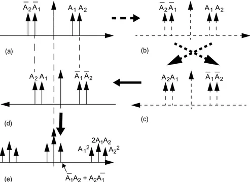
As an example, the output spectrum of a two-tone test signal in quadratic nonlinearity can be calculated as follows. The two-tone signal is given by

(2.7)

that is presented in Figure 2.8(a) using a two-sided spectrum. The right-hand side of the plot represents the positive frequency axis, and A₁and A₂ are now complex numbers containing both the amplitudes (A_j/2) and phases of lower (ω₁) and higher (ω₂) tones, respectively. Due to odd phase response of real systems, the phasorsA₁andA₂of the negative frequencies on the left are complex conjugates of A₁and A₂. Figure 2.8(b) is identical to Figure 2.8(a), whereas Figure 2.8(c) presents the original input spectrum with a reversed frequency axis: Positive frequencies are now on the left and negative frequencies on the right. Next, the reversed spectrum is slid from right to left and compared at all offsets to the original input in Figure

h t( )*x t( ) h( )τ x t( –τ) τd ∞

– ∞

∫

=

y t( ) = x t( )⋅x t( )↔ Y j( ω) = X j( ω)*X j( ω)

x = A₁⋅ cos(ω₁t+φ₁)+ A₂⋅cos(ω₂t+φ₂) A₁ejφ1

2

---⋅ejω1t A1e j – φ₁ 2

---⋅e–jω1t +

=

A₂ejφ2 2

---⋅ejω2t A2e j – φ₂ 2

---⋅e–jω2t +

(32)

2.8(a). Figure 2.8(d) presents the situation at a single frequency offset, that corresponds to a single frequency in the output spectrum. Now we simply multiply all the aligning frequency pairs [shown with dashed line between Figure 2.8(a, d)] and place the sum of these products (A₁A₂+A₂A₁) as the amplitude (actually a phasor) of the generated tone. The frequency offset between Figure 2.8(a), (d) corresponds to the envelope frequency f₂–f₁ (also called the beat, video, or modulation frequency), but the other tones are generated similarly. For example, a frequency offset 2ω₁[i.e., the origin of the spectrum Figure 2.8(d) aligns with frequency 2ω₁ in the original spectrum Figure 2.8(a)] causes theA₁phasors in Figure 2.8(a), (d) to align, resulting in a second harmonic with amplitudeA₁2in spectrum (e). Finally, Figure 2.8(e) presents the complete spectrum generated by squaring the two-tone signal in Figure 2.8(a). The procedure demonstrated in Figure 2.8 is known as spectral convolution.

Note that it is necessary to use a two-sided spectrum to calculate the amplitudes of the distortion tones using the spectral convolution. Hence, all amplitudes except the dc term include the term 1/2.

A₁A₂

A22

2A1A2

A12

A1A2 + A2A1

A₂A₁ A₁A₂

A1

A2 A1A2

A₁

A₂ A1A2

(a) (b)

(c) (d)

(e)

Figure 2.8 Spectral convolution. (a) The original and (b)-(c) flipped spectrum; (d) shows the flipped and shifted spectrum, and (e) is the final convolution result. Note that the phasors include the coefficient 1/2.

(33)

Some Circuit Theory and Terminology 21 2.3Memoryless Spectral Regrowth

This section discusses the spectral regrowth in a memoryless nonlinearity. A block presentation of a nonlinear system modeled by an input-output polynomial (2.3) is given in Figure 2.9, where the output is the sum of the first, second, and third powers y₁,y₂, and y₃ of the input signal, weighted by the nonlinearity coefficients a₁, a₂, and a₃, respectively. In phasor analysis, the coefficients may be complex to model the phase shift in the nonlinearities. The spectrums in the intermediate points A and B can be calculated as a two- and three-fold convolution of the two-sided input spectrum, respectively. As an example, the line spectrum of a squared two-tone signal in point A is shown in Figure 2.8(e).

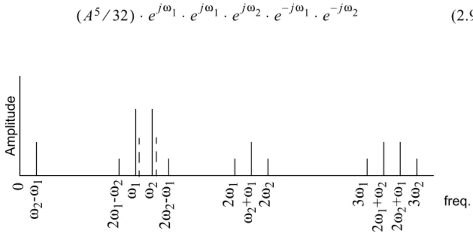
This polynomial system is usually analyzed by assuming that x(t) is a nondistorted two-tone signal. In this case, the linear terma₁xjust amplifies the fundamental tones at ω₁ and ω₂ (ω₂>ω₁). The quadratic nonlinearity a₂x2 rectifies the signal down to dc band to frequencies 0 Hz (dc) and ω₂–ω₁. It also generates the second harmonic band consisting of tones at 2ω₁, 2ω₂andω₁+ω₂, called the lower and higher second harmonic and the sum frequency, respectively. Similarly, the cubic nonlinearity a₃x3 generates lower and higher IM3 at 2ω₁–ω₂, and 2ω₂–ω₁ and the compression/expansion terms (AM-AM) on top of the fundamental tones ω₁andω₂, all appearing in the fundamental signal band. It also generates the entire third harmonic band consisting of tones at 3ω₁, 2ω₁+ω₂, ω₁+2ω₂, and 3ω₂, called the lower third harmonic, the lower and higher sum frequencies and the higher third harmonic, respectively. These tones are illustrated in the line spectrum shown in Figure 2.10.

Distortion tones are classified as harmonic (HD) and intermodulation (IM) distortion, where the harmonic distortion is simply an integer multiple of one of the input tones and IM tones appear at frequencies

x(t) y(t)

y1(t)

y₃(t) y₂(t) a1

a2

a₃ A

B

(34)

Kω₁+Lω₂, (2.8)

where K and L are positive or negative integers. Another, more practical classification is based on the grouping of the tones: in RF applications, the dc, fundamental, second and third harmonic bands are far from each other and quite easily filtered separately, if needed. However, the IM3 distortion appearing in the fundamental band cannot usually be separated from the desired linear term.

The third and the most important classification is based on the order of the distortion product, which in short means the number of fundamental tones that need to be multiplied to make a distortion product of a given order. In a two-tone excitation in Figure 2.10, the fundamental tonesω₁and ω2 are first-order signals, while dc (0 Hz), envelope ω2–ω1, second harmonics 2ω₁ and 2ω₂, and the sum frequency ω₁+ω₂ are second-order signals. These build up the dc and second harmonic bands. Similarly, third-order signal components lay in the fundamental (2ω₁–ω₂,ω₁,ω₂, 2ω₂–ω₁) and third harmonic bands (3ω₁, 2ω₁+ω₂,ω₁+2ω₂, 3ω₂). The amplitudes of theNth-order tones always are proportional toAN, whereAis the amplitude of the fundamental tone(s).

Using the notations of (2.8), the order N is sometimes written as N= |K|+|L|. However, this rule breaks down when higher order tones fall on top of the lower order ones. As an example, look at the fifth-order compression term (2.9) below that appears at frequency 1ω₁+0ω₂but still is of the fifth order.

(2.9)

freq.

Amplitude

ω2 ω1 2ω1

-ω2

2ω2

-ω1 ω2

-ω1

0

2ω

2

+

ω1

2ω

1

+

ω2 3ω1 3ω2 ω2

+

ω1 2ω1 2ω2

Figure 2.10 Spectral regrowth of a two-tone signal. AM-AM is shown as a dashed line next to fundamental tones.

A5⁄32

(35)

Some Circuit Theory and Terminology 23 Then what is the difference between the order of distortion and the degree of nonlinearity? So far the input signal has always consisted of first-order signals only, and the things have been simple: the first-degree term a₁xin (2.3) generates first-order tones, the second-degree (quadratic) term a₂x2 second-order tones, and the third-degree (cubic) term third-order tones. However, the case is not so simple any more, if the input signal is already distorted, which is the typical case inside a real amplifier. A second-degree nonlinearityx2essentially makes a productx₁x₂, where the x₁ and x₂ are certain input tones. These need not be the same, and their order may already be higher than one. For example, multiplying the fundamental tone ω₁ with a second harmonic 2ω₂ inside a second-degree nonlinearity generates two third-order tones at 2ω₂–ω₁ and 2ω₂+ω₁. Hence, the order of the output tone is the sum of the orders of the input tones x₁ and x₂. In one extreme, a purely quadratic (second-degree) nonlinearity is capable of generating any order of distortion, if the distorted output is always fed back to the input.

To summarize, the term order is a property of the final distortion product, and it is related to the amplitude dependency and frequency of the distortion tone. The term degree is a property of the nonlinear device, defining the shape of the nonlinearity. The order of the distortion caused by an Nth-degree nonlinearity depends both on the degree of the nonlinearity and the order of the input signals. In an Nth-degree nonlinearity, Ntones are multiplied, and the total order is the sum of the orders of theseN tones. This is illustrated in Table 2.4, where the amplitudes of all the tones generated by a third-degree polynomial are shown in a case where the input signal is a sum of the fundamental two-tone signal with phasorsA₁and A₂ and the second-order distortion tones DC, E, H₁₁, H₁₂, and H₂₂ at frequencies 0, ω₂–ω₁, 2ω₁, ω₁+ω₂, and 2ω₂, respectively.We see that in this case, also the second-degree (quadratic) nonlinearitya₂x2can generate third-order distortion appearing at the fundamental and third harmonic bands.

(36)

Table 2.4

Spectral components generated in a third-degree polynomial nonlinearity y =a₁x +a₂x2 +a₃x3 for a sum of two-tone signal phasorsA₁ andA₂ and second-order distortion phasorsE,H₁₁,H₂₂, andH₁₂ atω₂–ω₁, 2ω₁, 2ω₂, andω₁+ω₂, respectively. The terms inside the boxes present the third-order

results generated from first and second-order signals in the input.

Frequency Name a₁x (a₂ / 2)x (a₃ / 4)x

0 DC DC A₁A₁+A₂A₂

envelope E 2A₁A₂

IM3L EA₁+H₁₁A₂ 3A₁2_A

2

FUNDL A1 EA2+H11A1+

2DCA₁+H₁₂A₂ 6A1A2A2+3A1A1A1 FUNDH A₂ EA1+H22A2+

2DCA₂+H₁₂A₁ 6A1A1A2+3A2A2A2

IM3L EA₂+H₂₂A₁ 3A₁A₂2

2HL H₁₁ A₁2

2SUM H₁₂ 2A₁A₂

2HH H₂₂ A₂2

3HL H₁₁A₁ A₁3

3SUML H₁₁A₂+H₁₂A₁ 3A₁2_A

2

3SUMH H₂₂A₁+H₁₂A₂ 3A₁A₂2

3HH H₂₂A₂ A₂3

ω₂–ω₁

2ω₁–ω₂ ω₁

ω₂

2ω₂–ω₁ 2ω₁ ω₁+ω₂

2ω₂ 3ω₁ 2ω₁+ω₂ 2ω₂+ω₁

(37)

Some Circuit Theory and Terminology 25 2.4 Signal Bandwidth Dependent Nonlinear Effects

Section 2.1 described the classification of electrical systems into linear and nonlinear systems with and without memory. This classification is presented graphically in Figure 2.11, in which the overlapping segment between two areas represents nonlinear systems with memory. This segment is further subdivided into two sections. The upper section represents a narrowband system, where the transfer function is dependent on the center frequency of the system only, while the lower section represents a system that is also affected by the bandwidth of the input signal. Since all practical systems are more or less affected by signal bandwidth, the upper section is referred to as a narrowband approximation of a real, bandwidth-dependent system. In this book, bandwidth-dependent effects are called memory effects.

The narrowband single-tone signal used in Section 2.1 is insufficient for the characterization of memory effects. Instead, these effects can be investigated by applying a two-tone input signal with variable tone spacing. The alternative would be to use a real, digitally modulated signal, but it would yield less insight in the operation of the analyzed system, as will be seen later on. In addition, using a digitally modulated signal for the calculation of generated spectral components necessitates a time domain analysis tool with a Fourier transformation. The use of a sinusoidal input signal circumvents this problem, because spectral components can be calculated analytically.

This book studies the effects of variable tone spacing in detail to characterize bandwidth-dependent effects. Applying a two-tone signal to a third-degree polynomial system (2.3) results in the following two

nonlinear systems systems with memory

AM-AM conversion

AM-PM conversion Memory effects

energy storing circuit elements

Figure 2.11 Definition of memory effects used in this book. From [3].

v_C 1 C ---- i td

∞

–

t

∫

(38)

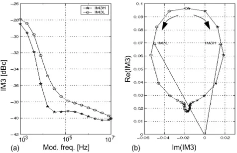
conclusions concerning IM3 signals at the output: first, they are not functions of tone spacing and, second, their amplitude increases exactly to the third power of the input amplitude. This is shown by the last column and third row in Table 2.4. The equation for the IM3L (lower IM3) component is proportional to the power of three while being independent of signal bandwidth. However, a comparison between the polynomially modeled and actual phases of the IM3L as a function of tone difference in a two-tone signal is sketched in Figure 2.12, where large differences can be observed between the two. The real phase (and amplitude) of the IM3 may deviate at low and high tone spacings (or modulation frequencies), indicating the existence of signal bandwidth-dependent nonlinear effects with memory, as marked by the lower overlapping area in Figure 2.11. This book refers to such effects as memory effects, and distinguishes between two distinct types: electrothermal memory effects, which typically appear at low modulation frequencies (below 100 kHz), and electrical memory effects appearing above MHz modulation frequencies.

The fundamental output of a two-tone input is also modified by a third-degree nonlinearity, shown in Figure 2.10 and Table 2.4. As a result, the two-tone signals are also affected by the amplitude and phase conversions. It then follows that memory effects can be characterized as changes in these conversions produced by a varying two-tone input [6]. Unfortunately, a two-tone input is hampered by the same drawbacks as a one-tone input. Strong linear signals at the fundamental make nonlinear effects difficult to measure. This is particularly important in the characterization of memory effects, which are usually very weak compared to linear signals. Therefore, the analysis of intermodulation components is the most practical starting point for the exploration of memory effects.

tone spacing (ω2-ω1) polynomial input-output system

electrical

pha(IM3L)

system with memory effects electrothermal

(39)

Some Circuit Theory and Terminology 27 2.5 Analysis of Nonlinear Systems

Most nonlinear analysis/simulation methods operate either fully or partially in the time domain. Standard transient analysis based on numerical solving of nonlinear differential equations is an example of the former, and widely used harmonic balance method presents the latter. Here the passive components are modeled in the frequency domain, but still the responses of the nonlinear components are solved in time domain, and outputs and excitations are pumped back and forth between time and frequency domain using the discrete Fourier transform. Transient analysis can handle any form of input signal or even autonomous circuits (oscillators), but it suffers from ineffective modeling of distributed components and long-lasting initial transients that need to settle before the steady-state spectrum can be calculated. In the harmonic balance the signal is necessarily modeled by just a few sinusoids, but the initial transient is bypassed and more accurate frequency domain models can be used for passive components. An in-depth comparison of the basic simulation algorithms can be found in [7].

The Volterra analysis technique used in this book is calculated entirely in the frequency domain, building higher order responses recursively using lower order results. Hence, no iteration is needed and it is a very quick and RF-oriented analysis method. What is even more important in studying the memory effects is that it can separate the sources of distortion exactly in the same way engineers are accustomed to doing in noise simulations: The dominant contributions can be listed, and the designer can attack them first. That kind of information is very valuable for design optimization, but usually impossible to derive from transient or harmonic balance simulations that usually display only the total amount of distortion.

In the Volterra analysis, some simplifications and assumptions are made, though. The first simplification is that like in harmonic balance, only the sinusoidal steady-state response of a single or two-tone excitation is calculated. Second, the nonlinearities of the system are modeled polynomially (2.3). Using these assumptions, we may apply the Volterra method for calculating the output of a nonlinear system, which can give either numerical or analytical results for the distortion components.

(40)

2.5.1 Volterra Series Analysis

Volterra analysis can be considered a nonlinear extension of linear ac analysis, and its main difference compared to the often-used power series analysis is that it contains also the phase information of the transfer functions. It is often calculated symbolically [8-11], in which case the transfer functions describing the amplitude and phase of the distortion tones as functions of input signals are derived. These transfer functions are illustrated in Figure 2.13(a), where H₁ is the linear (small-signal) transfer function, H₂ is the second-order transfer function (producing all the second-order tones in a two-tone test), and so forth; the total outputy(t) is a sum of all these transfer functions applied to the input signalx(t) [8,12,13]. The difference between linear and Volterra analysis is further illustrated in Figure 2.13(b). Linear small-signal ac analysis models thex-y input-output characteristic of a circuit element with its first derivative in the operating bias point. In Volterra analysis, the actual shape of the I-V or Q-V curve is modeled by a best fit, low-degree polynomial function of the controlling voltage, and the higher-degree coefficients of the polynomial are used to calculate the distortion components.

The output of the second-order Volterra kernel for the one-tone sinewave (2.2) is derived in Appendix A for interested readers. However, since the spectral components at the output can be calculated using the direct calculation method explained in the next section, an in-depth understanding of Volterra kernels is beyond the scope of this book. In a

actual small-signal Volterra

x y

bias point H1

H2

H3

y(t) x(t)

(b) (a)

(41)

Some Circuit Theory and Terminology 29 fully numerical form, Volterra analysis has been implemented for example, in SPICE [14] and Voltaire XL [15] circuit simulators.

A word of warning concerning the Volterra analysis is needed. First, the polynomial models are notorious for the fact that their response explodes outside the fitting range -hence, the model is only locally fitted around the desired bias point and applicable over a certain amplitude range. The applicable range depends on the fitting range of the polynomial (as anything can happen outside the fitting range), the nonlinearity of the device, and the degree of the modeling polynomial. As the degree of the model always needs to be limited at some rather low degree, some truncation error between the actual and the modeled response exists. The effects of this truncation error are discussed in some more detail in Appendix B.

Figure 2.13 and the block diagram in Figure 2.9 model only an input-output nonlinearity. Due to intentional or nonintentional feedback, most of the controlling nodes in real amplifiers also contain distortion components and not just the linear contribution. This causes multiple mixing, as already pointed out in Table 2.4. For example, the second harmonic may mix with the linear term in a second-degree nonlinearity and generate IM3. These effects can be taken into account as well, by keeping track of the order of the calculated result. If v₁ contains all linear and v₂ contains all second-order voltage phasors and so forth,v₁+v₂+v₃+... can now be substituted into the polynomial as shown in (2.10). After expanding this we can collect the terms of a given order on separate rows, and the last complete row in (2.10) shows that the third-order output currenti actually consists of three terms: input third-order distortionv₃(if present) multiplied by the linear gain a₁, input linear signalv₁distorted in the cubic nonlinearitya₃x3, and finally, a mixing result of linear and second-order input signalsv₁and v_2,generated in the quadratic nonlinearitya₂x2. Also, higher order terms likev₂2orv₃v₂ are generated, but they are ignored in this analysis.

(2.10) i = a₁(v₁+v₂+...)+a₂(v₁+v₂+...)2+a₃⋅(v₁+v₂+...)3

a₁v₁ =

a₁v₂ a₂v₁2

+ +

a₁v

3 a3v13 2a2v1v2

+ + +

(42)

2.5.2 Direct Calculation of Nonlinear Responses

A thorough study of the Volterra series can be found in [11, 13], while this book focuses on the frequency domain analysis only. Furthermore, rather than determining all third-order products, researchers usually concentrate on IM3 responses, which makes it impractical to derive the general form Nth-order Volterra kernels. Instead, the direct method [11], also known as the nonlinear current method, can be employed to calculate only the desired signal components.

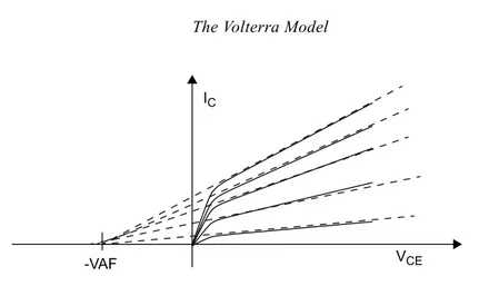
The direct method is based on modeling the nonlinear I-V and Q-V characteristics given by the polynomial functions in Figure 2.14 with a parallel combination of a linear element and a nonlinear current source, the current of which depends on the polynomial coefficients and the controlling voltages. This is illustrated in Figure 2.14, whereK_1GtoK_3Gmodel the I-V and K_1C to K_3C the Q-V characteristic curves of a nonlinear conductance and capacitance, respectively. The linear terms K_1G and K_1C are modeled by a linear conductance and capacitance, and the higher degree nonlinearities are modeled by nonlinear voltage-controlled current sources. Furthermore, as the Q-V polynomial models the charge, it has to be differentiated with time to get the ac current. Note that the control voltagev may include also distortion voltages, which results in multiple mixing mechanisms, as illustrated in (2.10) and Table 2.4.

The procedure for the calculation of the response to a two-tone signal can be summarized as follows:

Figure 2.14 Equivalent models for nonlinear (a) conductance and (b) capacitance. i = K_1Gv+K_2Gv2+K_3Gv3

+

-v

+

-v i

t

∂∂(K1Cv+K2Cv2+K3Cv3) =

(43)

Some Circuit Theory and Terminology 31 1. Evaluate the fundamental (first-order) node voltages using linear ac

analysis for both tones.

2. For each nonlinear component, evaluate the second-order distortion currents using the fundamental voltage amplitudes. These will appear at five sum and difference frequencies: dc, envelope ω₂–ω₁, second harmonics 2ω₂, 2ω₁, and sum frequencyω₂+ω₁.

3. Use these distortion currents to calculate the second-order distortion voltages in each node using the ac analysis. Note that the distortion voltages are deterministic signals and they are summed as vectors, not as powers as in noise analysis.

4. Using the first- and second-order voltages, calculate the third-order distortion currents in the nonlinear components. These will appear at eight frequencies, two of which are IM3 signals.

5. Perform the ac analysis again at the frequencies of the third-order distortion currents to find the third-order node voltages.

In short, the linear node voltages are solved first, using small-signal analysis. Then, nonlinear analysis is started by modeling the nonlinearities by current sources and short (open)-circuiting the linear voltage (current) sources. Using linear analysis again, the second-order voltage responses of the distortion currents are calculated, and the procedure can be repeated all the way to higher order responses. An example of the direct calculation method will be given later on in this chapter.

Since the nonlinearities of the circuit elements are modeled by current sources, they will be explained in more detail. Each nonlinearity in the circuit is represented by a current source, which is placed in parallel with a linearized small signal element. The second-order current sources are calculated on the basis of the two-tone test signal, and the values of the second-order current source (one-sided) amplitudes at the envelope ω₁–ω₂ the second harmonic frequencies 2ω₁are given in Table 2.5 and those for the IM3 results in Table 2.6. Note that Table 2.6 from [11] does not give the AM-AM term of the fundamental tones or third harmonics, but these can be derived using Table 2.4.

(44)

necessary to make the envelope frequencyω₁–ω₂. If a negative frequency is needed, the voltage phasor for it is the complex conjugate of the phasor at the positive frequency.

The conductances are memoryless, but as i=dq/dt, the charge polynomial needs to be differentiated with respect to time, and this causes the jω dependency in the nonlinear current of capacitances. Hence, capacitors cause very small distortion currents at low frequencies, but high currents at the harmonic bands. A two-dimensional conductance is controlled by voltages v_iand v_j (e.g.,v_be and v_ce). Here, both controlling voltages need to have one-dimensional polynomials of their own, but there are also terms consisting of the cross-products of voltages on both ports. These additional cross-terms are listed in the tables.

Note again that the phase of negative frequency components is opposite to positive frequencies (i.e., V_i,-1,0 = V_i,1,0). Normal rules of complex arithmetic apply, and for example,c2 is still a complex number with twice the phase angle and frequency ofc, while |c|2₌_cc_{is a scalar real number at} dc. Some care is needed in calculating the responses of IM products consisting of both positive and negative frequencies, as terms v_in3 and v_in2v_in= |v_in|2_v

inhave different phase angles and frequencies, even though their amplitudes are exactly equal.

As seen from Table 2.6, the third-order signal components are not just functions of cubic nonlinearities, but they are also affected by the second-order voltages and quadratic nonlinearities. For example, the distortion current i_NL generated by a nonlinear conductance at the higher IM3 frequency 2ω₂–ω₁ has the amplitude and phase given by