www.elsevier.nl / locate / econbase
Extended benefits and the duration of UI spells: evidence
from the New Jersey extended benefit program
a,c b,c ,*
David Card , Phillip B. Levine a
University of California at Berkeley, Berkeley, CA, USA b
Department of Economics, Wellesley College, Wellesley, MA 02481, USA c
National Bureau of Economic Research, Cambridge, MA, USA
Abstract
This paper examines the impact on the duration of unemployment insurance receipt of a politically motivated program that offered 13 weeks of ‘extended benefits’ for 6 months in 1996. Using state-level data and individual administrative records from before, during and after the program, we find that it raised the fraction of claimants who exhausted their regular benefits by 1–3 percentage points. Had the program run long enough to affect claimants from the first day of their spell, the fraction exhausting would have risen by 7 percentage points, and the average recipient would have collected regular benefits for one
extra week. 2000 Elsevier Science S.A. All rights reserved.
Keywords: Unemployment insurance; Spell duration; Extended benefits
JEL classification: J64; J65
1. Introduction
One of the key factors that may explain some of the significant gap between European and American unemployment rates is the relative generosity of un-employment benefits. Although benefit levels tend to be somewhat higher in Europe, there is a much larger difference in the maximum duration of unemploy-ment benefits. In the United States unemployunemploy-ment insurance (UI) is typically
*Corresponding author. Tel.:11-781-283-2162; fax:11-781-283-2177.
E-mail address: [email protected] (P.B. Levine).
available for a maximum of 26 weeks, while in many European countries the maximum duration of unemployment benefits is measured in years. Conventional economic models suggest that the availability of longer UI benefits provides incentives for individuals to remain unemployed longer, contributing to the
1
problems of high unemployment and long-term joblessness.
In fact, existing research in the United States finds a strong positive relationship between the maximum duration of benefits and the length of an individual’s spell
2
of unemployment benefits. Empirical identification in this body of work is provided by differences in the maximum duration that occur across states and over time. A potential difficulty with this identification strategy is that states may decide to offer longer UI benefit durations during recessions, in response to low
3
rates of job-finding that cause more individuals to exhaust their benefits. Such endogenous policy formation may lead to an overstatement of the effect of longer UI benefits on the duration of UI spells.
In this paper we use the experiences generated by a unique legislative episode in the state of New Jersey that led to the adoption of extended unemployment
4
benefits for a 25-week period beginning on June 2, 1996. Since 1993, New Jersey had been using funds from its Unemployment Insurance Trust Fund to finance the indigent care costs of hospitals in the state. In the Spring of 1996, opponents of this financing method blocked its re-authorization, precipitating a legislative crisis. In a deal struck to gain the support of labor organizations, a law passed in May of 1996 included the provision of up to 13 weeks of ‘extended’ benefits for workers who exhausted their ‘regular’ UI benefits (those to which they are normally entitled — typically 26 weeks). These benefits were available retrospectively to claimants whose benefits had expired as long ago as December 1995, and prospectively to claimants who exhausted their regular UI benefits until November 24, 1996.
This policy change provides two important advantages for a study of the effect of maximum benefit durations on the length of unemployment spells. First, its legislative history makes the benefit extension unrelated to changes in the condition of the state’s labor market. New Jersey’s economy remained robust
1
See Nickell and Layard (1999) and Machin and Manning (1999) for discussions of long-term unemployment in Europe and the contribution of unemployment benefits to this phenomenon.
2
See, for example, Moffitt and Nicholson (1982), Moffitt (1985), and Katz and Meyer (1990a). This literature focuses on the narrow public finance question regarding the impact of maximum benefit duration on compensated unemployment spell lengths, not on total unemployment, due to data availability. For similar reasons, the research presented in this paper also focuses on this narrower question. If one had access to similarly complete micro-data on unemployment spells, an analysis of these hypothetical data would better address differences in total unemployment rates across countries.
3
Indeed, the federally funded extended benefit program is automatically triggered when insured unemployment rates reach a certain threshold. The fact that benefits are typically extended during a recession would not bias the results if the econometric model controlled for the determinants of the extension (like the insured unemployment rate).
4
throughout the period, with overall unemployment rates drifting down at about the same rate as in nearby states. Second, the short-term nature of the New Jersey Extended Benefit (NJEB) program allows us to compare unemployment spell durations and other outcomes during the program period with comparable data from immediately before and immediately after the NJEB interval.
We use two complementary sources of data for our analysis. We begin by studying aggregated monthly data for New Jersey and other states on the fraction of UI claimants who exhaust their regular UI entitlement. Standard evaluation techniques provide two estimates of the effect of the NJEB program: one effect when the program ‘turned on’; and a second when the program ‘turned off’. Our second data source is administrative claim records from the state of New Jersey from 1995 (the year before the NJEB program) to 1997 (the year after). We use these records to compare regular UI spell durations in the program period to spell durations before and after. An important feature of the NJEB program is that almost all potential recipients of extended benefits had begun their UI spells before the benefit extension was announced. Standard hazard-modeling techniques allow us to compare rates of leaving UI before and after the announcement of the NJEB program among these ongoing spells.
Our findings suggest that the NJEB program, as enacted, had a very modest effect on overall UI claim characteristics. Our aggregate and micro-level estimates indicate a 1–3 percentage point increase in the fraction of claimants who exhausted their regular UI eligibility. The impact of the policy, however, appears to have been substantially moderated by its short-term nature. Many recipients were well into their unemployment spell at the time the extension was im-plemented and had little opportunity to alter their behavior. Our hazard models suggest that the regular UI-leaving rate declined substantially (by about 15%) following the program’s introduction. Simulations of the long-term effect of a benefit extension similar to the NJEB program indicate that the availability of 13 extra weeks of benefits would raise the fraction of claimants who exhaust regular UI benefits by 7 percentage points, and would raise the average duration of regular UI claims by about 1 week.
2. Review of the literature
There are two sources of variability in maximum UI spell durations, neither of which necessarily provides exogenous changes in the duration of benefits. At the aggregate level, policy changes (enacted by federal or state governments) alter the duration of benefits for all claimants. The problem with these changes is that they are almost always triggered by slackness in the labor market that has lead to high unemployment rates, leading to a potential reversal of causality. At the individual level, differences in past labor market histories create differences in the maximum amount of time that different individuals can receive UI. The formula that converts differences in labor market histories into different entitlement periods varies across states, providing some geographic variation in maximum benefit length. However, to the extent that differences in UI entitlement are correlated with (or caused by) unobserved individual characteristics that also affect UI-leaving rates, variation in individual-specific UI benefit durations is problematic.
Perhaps the most convincing evidence that job-finding behavior is influenced by the maximum duration of benefits comes from an examination of the rate of leaving the UI roles in the weeks before benefit exhaustion (cf. Meyer, 1990; Katz and Meyer, 1990b). The available data clearly indicate that the probability of leaving UI (the hazard rate) rises sharply in the last few weeks of benefit eligibility. Although this evidence is strongly suggestive that some individuals search harder to find a job (or return to pre-arranged jobs) just prior to benefit exhaustion, it does not directly address the policy question of the impact of a benefit extension on exit rates from UI. Moreover, results in Meyer (1990) suggest that individuals who were already collecting UI at the time of a benefit extension also have a ‘spike’ in their UI-leaving rate prior to the time their benefits were previously scheduled to exhaust, even though they were eligible for longer benefits.
These concerns underscore the potential usefulness of studying the effect of a legislative change in maximum benefit durations that came about at a time of stable macroeconomic conditions, such as that generated by the NJEB program. We therefore turn to a detailed discussion of this program and its origins.
3. The New Jersey benefit extension
3.1. Overview of the UI system
The UI system in the United States is administered by the individual states under a set of national guidelines established by the federal government. Regular
5
UI benefits are financed through a payroll tax that is mainly levied on firms. Each state operates a UI Trust Fund that accumulates funds during expansionary years
5
in order to finance higher expenditures in economic downturns. UI taxes are partially ‘experience rated’: firms whose previous employees have drawn more benefits are taxed at higher rates, subject to (often binding) minimum and maximum rates.
Unemployed individuals are eligible to collect UI benefits if they have a sufficient work history and if they remain able, available, and actively seeking work. Weekly UI benefits are paid out according to an individual’s earnings history prior to job loss, subject to a minimum and maximum benefit. The maximum benefit rate varies tremendously across the states, ranging from $175 per week in
6
Missouri to $365 per week in the state of Washington in 1996. New Jersey is among the most generous states, providing a maximum benefit of $362 per week in 1996. In contrast to the interstate variation in benefit levels, almost all states, including New Jersey, specify a maximum entitlement period of 26 weeks during
7
normal economic conditions.
Although regular UI benefits are usually available for up to 26 weeks, the maximum duration of benefits is sometimes extended in cyclical downturns. In fact, since 1970 there has been a federal program that provides 13 weeks of extended benefits when a state’s insured unemployment rate (the number of current UI claimants divided by the number of employed workers covered by the system) exceeds a specific threshold. Changes in the UI system over time, however, have made the trigger virtually unattainable (Blank and Card, 1991), and over the past two decades federal emergency legislation has been enacted on an ad hoc basis to provide extended benefits during recessions (Blaustein et al., 1993; Woodbury and Murray, 1997). In addition, individual states can (and sometime do) raise the maximum duration of benefits. To the best of our knowledge, such increases have occurred exclusively during periods of adverse labor market conditions.
3.2. ‘Charity care’ and the New Jersey benefit extension
In contrast to the traditional pattern of linking UI benefit extensions to changes in labor market conditions, the NJEB program emerged from a political com-promise around the state’s ‘Charity Care’ program for indigent hospital patients. Since its inception in 1987, the financing of this program was controversial, and over its 10-year history state legislators struggled to devise alternative financing
6
These benefit levels are exclusive of dependent’s allowances which are available in some states. The additional payments made for each child is small in each of the handful of states which offers them.
7
arrangements. We detail some of this turbulent history here because it illustrates how the 1996 benefit extension came about as a short-run solution to a political dilemma.
In its original formulation the New Jersey Charity Care program was funded by the Uncompensated Care Trust Fund, which collected a 19% surcharge on the hospital bills of paying patients. Soon after its introduction the surcharge came under fire for driving up hospital rates and insurance premiums, and lowering the number of individuals covered by insurance. Legislative extensions of the program became hotly contested and the program even expired briefly in 1989 and 1991, only to be revived shortly thereafter. In 1992, a lawsuit successfully challenged the surcharge tax, ending this method of financing.
To replace the revenues from the surcharge, state legislators agreed to finance Charity Care by diverting some of the surplus available in New Jersey’s Unemployment Insurance Trust Fund. This plan was very unpopular among both labor and business groups. Labor groups worried that using funds from the Trust Fund would reduce the benefits available to unemployed workers in the future. Business groups viewed the plan as a hidden payroll tax. Despite these concerns, the Charity Care program was funded in this manner from 1993 to the end of 1995, when opposition grew strong enough to block an extension. However, none of the alternatives proposed at the time, including a payroll tax, a tax on health insurance premiums, a tax on revenues from video poker games, and a rise in the tobacco tax, could garner enough support to be enacted. The resulting legislative gridlock led the Charity Care program to expire at the end of 1995.
Through the early months of 1996 legislators tried in vain to find ways to reinstate the program. One proposal to break the deadlock was to continue drawing funds from the UI trust fund, but, in a gesture to organized labor, to authorize a short-term extension in the maximum duration of UI benefits. The first reference we have found to this proposal appears in a single sentence near the end of a New
York Times article (March 3) on the financing crisis. Support for the proposal grew
as the crisis continued; hospitals received their last payment for indigent care in February and were warning of layoffs and possible hospital closures if the issue was not resolved quickly. In the middle of May, legislation was enacted that, among other things, traded a benefit extension for the continued use of the UI trust
8
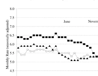
fund to 1997. By the end of 1997, new legislation was enacted that gradually eliminates the reliance on the UI trust fund by 2003, increasing the tax on cigarettes and appropriating general revenues to cover the remainder of the cost. An examination of patterns in labor market activity by state demonstrates that the NJEB program was unrelated to changes in business cycle conditions. Fig. 1 displays unemployment rates in New Jersey, Pennsylvania and for the entire
8
Fig. 1. Monthly unemployment rate.
9
United States. Recall that the period in which NJEB was in effect was June– November of 1996. Unemployment held roughly constant in New Jersey and much of the rest of the country in 1995 before falling in 1996 and 1997. New Jersey’s economy appeared to grow more quickly than the US as a whole over this period, but no noticeable break from trend is apparent within New Jersey or between New Jersey and other states around the period in which NJEB was in effect. As one might expect based on the legislative history, no obvious relationship exists between changes in business cycle activity and the timing of the NJEB program.
3.3. Provisions of NJEB
The specific provisions of the benefit extension included a 50% increase in the number of weeks for which benefits could be received, equivalent to a 13-week
9
extension for the large majority of recipients who were eligible for 26 weeks of regular benefits. The extension was available to all recipients who exhausted their regular UI benefits between June 2 and November 24 of 1996. The policy also applied retrospectively to the set of claimants whose benefits expired as far back as December 2 of 1995, which we subsequently refer to as the ‘reachback’ group.
To collect these benefits, an exhaustee needed to return to the UI office to file a separate claim for the extension. Formal notification letters were sent to in-dividuals in the ‘reachback’ group who had exhausted their benefits soon after the legislation was enacted. Claimants currently receiving UI, and those who started a new claim after June 2, were not individually notified of the benefit extension until they received their final regular UI benefit payment. However, the state UI agency engaged in a variety of outreach activities, including press releases, meetings with union officials, and the like. In addition, the notification of the reachback group presumably generated word-of-mouth dissemination, particularly among frequent users of the UI system.
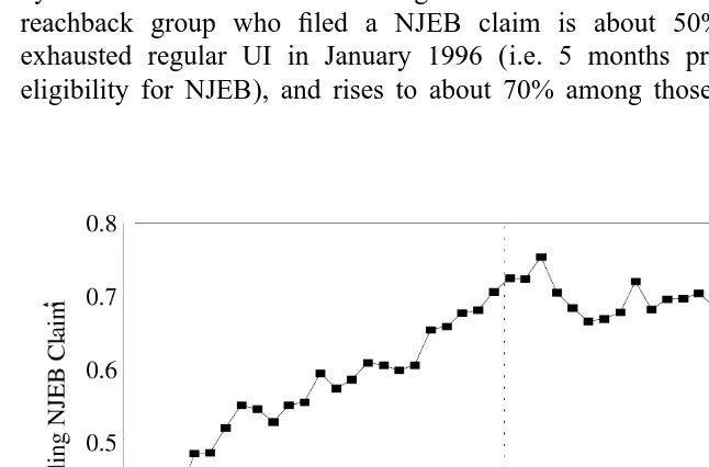
Fig. 2 displays the take-up rate of NJEB benefits among eligible UI recipients by the month of exhaustion of regular UI benefits. The fraction of those in the reachback group who filed a NJEB claim is about 50% among those who exhausted regular UI in January 1996 (i.e. 5 months prior to notification of eligibility for NJEB), and rises to about 70% among those who exhausted their
10
regular benefits just prior to the law’s enactment. The take-up rate for later
claimants (i.e. those who exhausted after the effective date of the law) remains fairly steady at about 70% — a rate similar to estimates of the take-up rate for regular UI benefits among eligible job losers (see, for example, McCall, 1995;
11
Anderson and Meyer, 1997).
Nevertheless, the fact that 30% of eligible recipients did not claim NJEB raises an issue regarding the interpretation of the results presented here. If eligible individuals did not take up benefits because they did not know about their availability, then estimates of the behavioral response to the program would be biased downwards, relative to the expected responses from a more widely advertised program. We believe that this bias is unlikely to be severe, however. First, the program dissemination and application processes were similar to those used in other benefit extensions in New Jersey, including Emergency Unemploy-ment Compensation in the early 1990s. Although that program, in particular, did generate higher take-up rates than NJEB according to New Jersey officials, it was also offered during a recession. Evidence indicates that the most common reason for not applying for regular benefits among those who are eligible is the expectation of finding a job soon (Vroman, 1991; Anderson and Meyer, 1997). Such expectations are no doubt more likely when economic conditions are favorable and probably affect the decision to file for extended benefits as well. Second, representatives of the New Jersey Department of Labor reported to us that within a few weeks of the program’s inception, recipients were well-informed about the benefit extension. In fact, in the few weeks following the expiration of the program on November 24, 1996, a substantial number of recipients registered complaints that they could not get it. In our empirical analysis, we investigate this potential source of bias further by separately examining groups of workers who
10
The relatively high take-up rate for NJEB among those who exhausted 6 months earlier is potentially surprising, and suggests that many of these individuals had not found work even after 12 months of joblessness.
11
were more likely to have full information regarding the program’s existence to see if their response is larger than that observed from other workers.
4. Empirical strategy and description of the data
The legislative history of the NJEB program makes it clear that the benefit extension was unrelated to changes in business cycle conditions in the state. Its introduction and ending create conditions that are ideal for a quasi-experimental analysis of the effect of maximum benefit durations on the behavior of UI claimants. In fact, the short-term nature of the policy provides two opportunities to examine the impact of higher benefit durations: one as the NJEB program began; and another when the program ended. Any effect measured at the onset of the program should dissipate at its expiration.
We use two different sources of data to evaluate the effects of the NJEB program. First, we obtained monthly data for the UI systems of all 50 states and the District of Columbia from January 1985 to October of 1997 from the US
12
Department of Labor. These state-level data contain information on the number
of initial UI claims and first payments, the fraction of claimants that exhaust their regular benefits, and the level of covered employment in each month over this period.
These data allow us to determine whether the rate of regular benefit exhaustion (defined as the number of exhaustions divided by the 6-month lag of first payments) increased and then returned to its previous level, during and after the
13
period in which New Jersey’s extended benefits were available. We test for the
presence of such a pattern in three ways: (1) by comparing exhaustion rates in New Jersey over time; (2) by comparing exhaustion rates in New Jersey with rates in neighboring Pennsylvania; and (3) by comparing exhaustion rates in New Jersey with those in the rest of the country.
Our second source of data is administrative records from New Jersey’s UI system for all initial claims filed between January of 1995 and December of 1997. Some 1.3 million claims were filed over this period, with first payments made to
12
At the time we obtained these data in the Spring of 1998, we could only create exhaustion rates for initial claims filed to October of 1997. Claims filed later than that had not hit their 6-month potential maximum duration yet. Therefore, we have no data for November of 1997 which would have been useful for comparison purposes with the NJEB window in 1996.
13
14
815 077 claimants. We restrict our attention to the subsample of claimants who
received a first payment, whose files include complete demographic and industry information, and who received no more than one week of partial UI benefits. The latter restriction is adopted to eliminate the small fraction of claimants who
15
worked part-time while they collected UI. We also exclude all claimants younger
than age 18 or older than 65, resulting in a useable sample of 701 743 UI recipients.
The estimation results reported in this paper are based on the subsample of 283 308 claimants whose regular UI benefits were scheduled to exhaust between July 1 and November 24 of 1995, 1996 or 1997. The period July 1–November 24, 1996 includes most of the claims that were prospectively eligible for NJEB, allowing a one-month lag for information about the program to disseminate among
16
claimants. We use data for those claimants scheduled to exhaust their regular
benefits from the same months of 1995 and 1997 as a ‘comparison period’, to hold constant the seasonal differences that exist in the composition of UI claimants and in job-finding behavior. For those scheduled to exhaust regular benefits within these three annual windows, job-finding activity in each week of their unemploy-ment spell is analyzed, not just those weeks within the July–November period.
It is important to note that our micro-sample is limited to New Jersey UI claims. We can only use this sample to make comparisons within New Jersey over time. Thus, an assumption in most of our micro-analysis is that claims from 1995 and 1997 form a valid ‘counterfactual’ for claims in 1996 (controlling for observable factors such as unemployment rates). We provide some limited evidence on the validity of this assumption below.
The individual claims micro-data can be used to refine our analysis of aggregate exhaustion rates — for example, by taking into account differences across claimants in the maximum duration of regular benefits. The more important use of the micro-data, however, is to estimate weekly hazard rates for ending a UI claim spell, and to measure the effect of NJEB eligibility on these hazard rates. Because
14
Individuals who file an initial claim but do not receive a first payment include those who find a job during the waiting week, who are deemed ineligible for benefits after filing a claim, or who find a job during the period in which eligibility is being determined among those for whom eligibility has been questioned.
15
See McCall (1996) for discussion of the set-aside provisions that allow UI recipients to work part-time and collect some benefits. We include claimants who collect one week of partial payments because recipients frequently obtain employment in the middle of the week and their last payment is a partial one. As discussed in more detail below, a limitation of the data available to us is that we cannot identify those respondents whose first weekly payment was a partial one.
16
of the limited timeframe of the NJEB program, the vast majority of UI claims
17
affected by NJEB were in progress in June 1996. The NJEB intervention
therefore affected different individuals differently, depending on how many weeks they had been on UI at the announcement of the program. Such a ‘time-varying’ intervention is most easily modeled in the context of a conventional hazard model. A second use of the individual claims data is to examine the effect of the NJEB program on the ‘spike’ in UI exit rates just prior to exhaustion of regular UI benefits. To the extent that this spike reflects a behavioral response to the impending cut-off in benefits, one might expect a smaller spike among claimants who were eligible for NJEB than among claimants in the comparison group. (Although, as noted earlier, Meyer (1990) did not find much evidence of such a change).
5. Results
5.1. Analysis of aggregate data
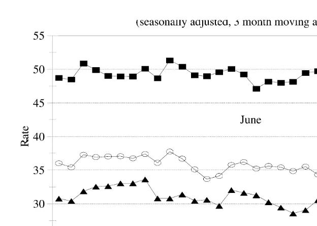
Fig. 3 graphs aggregate monthly exhaustion rates between 1995 and 1997 for New Jersey, Pennsylvania, and the entire United States. One obvious difference across these geographic entities is that the average exhaustion rate is higher in
18
New Jersey. The ratio of exhaustions to 6-month lagged first payments hovers
around 50% in New Jersey compared to roughly 30% for Pennsylvania and 35% for the country as a whole. Nevertheless, movements in exhaustion rates tend to
19
follow each other rather closely.
Beginning in June of 1996, however, New Jersey’s exhaustion rate began increasing slightly, while rates elsewhere drifted down. The New Jersey rate stood at about 48% in June before increasing to over 50% in November of 1996 for the first time in over a year. No such trend appears in Pennsylvania or in the national data. This relative upward trend is consistent with the expected effect of the NJEB program. In particular, one would expect the availability of NJEB to lead to a
17
An individual could file a claim after the June 2, 1996 date, NJEB became effective and still exhaust their regular benefits by November 24 of that year. For instance, an individual filing a claim on June 2 who was eligible for 22 or fewer weeks could still qualify for NJEB. The number of recipients for whom this is true is very small.
18
We graph 3-month backward-looking moving averages because the month-to-month variation in exhaustion rates is considerable, possibly overshadowing other patterns. Use of a moving average means that any policy effect will not be observed as a discrete break in the trend, but will be more gradual.
19
Fig. 3. Exhaustion rate for regular UI benefits in New Jersey, Pennsylvania and US.
lower exit rate from UI for workers who had just started UI claims, as well as for
20
those had been on UI for longer. Such behavior would lead to a gradual rise in
the exhaustion rate, with a plateau after 26 weeks, as all those who became eligible for NJEB while on UI eventually exhaust. Given the short timeframe of the NJEB program, one would therefore expect a monotonically rising effect throughout the June–November 1996 period. In the months after the benefit extension ended, exhaustions fell considerably in New Jersey, although a small decline is also observed in the US as a whole.
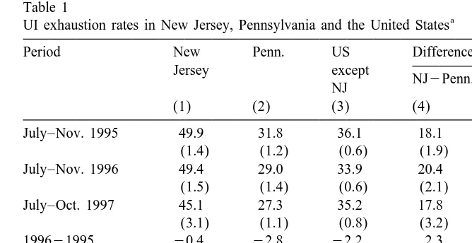
Simple estimates of the impact of NJEB can be obtained by computing the change in exhaustion rates in New Jersey relative to the change in other states as NJEB benefits ‘turn on’ and ‘turn off’. Such estimates are reported in Table 1. The first three columns of this table present exhaustion rates in New Jersey, Pennsylvania, and the US (excluding New Jersey) for the July–November periods
21
of 1995, 1996 and 1997. We use a July–November window rather than a June
20
Mortensen (1977) uses a simple search model to derive the predicted effects of longer benefit availability on search behavior of unemployed workers, and on the exit rates off UI.
21
Table 1
a UI exhaustion rates in New Jersey, Pennsylvania and the United States
Period New Penn. US Differences
Jersey except
NJ2Penn. NJ2US NJ
(1) (2) (3) (4) (5)
July–Nov. 1995 49.9 31.8 36.1 18.1 13.7
(1.4) (1.2) (0.6) (1.9) (1.5)
July–Nov. 1996 49.4 29.0 33.9 20.4 15.5
(1.5) (1.4) (0.6) (2.1) (1.6)
July–Oct. 1997 45.1 27.3 35.2 17.8 9.9
(3.1) (1.1) (0.8) (3.2) (3.2)
Standard errors in parentheses. Exhaustion rate represents the number of claims exhausting in a month divided by the number of first payments 6 months earlier. The averages reported for July–November are weighted averages of the respective months, using as weights the number of claims (lagged 6 months). The 199621995 and 199721996 differences are simple differences of the respective averages. The entries in the last row of the table represent the difference between the 1996 average and the simple average of the 1995 and 1997 averages. Data for November 1997 are unavailable.
starting date to allow for information lags during the first few weeks of the NJEB program. Columns (4) and (5) report the differences in exhaustion rates in New Jersey relative to the two comparison groups. As noted in Fig. 3, average exhaustion rates are higher in New Jersey than in Pennsylvania, and also higher than in the rest of the US as a whole.
The row labeled ‘199621995’ gives the change in exhaustion rates between the
1995 and 1996 periods, while the row labeled ‘199721996’ gives the change
from 1996 to 1997. The entries for these rows in columns (4) and (5) are the ‘differences-in-differences’ in exhaustion rates between New Jersey and either comparison group as NJEB started and ended. Finally, the last row of the table shows the difference in average exhaustion rate for July–November, 1996, relative to the average for the same months in 1995 and 1997.
A number of alternative estimates of the effect of the NJEB program on New Jersey exhaustion rates can be drawn from Table 1. For example, suppose that average exhaustion rates would have followed a linear trend in New Jersey from 1995 to 1997, in the absence of NJEB. In this case, the average of 1995 and 1997 exhaustion rates is a valid counterfactual for 1996. Under this assumption, NJEB raised exhaustion rates by about 2 percentage points.
Pennsylvania in the absence of the NJEB program. In this case, we have two estimates of the NJEB effect: a 2.3 percentage point estimate (from the com-parison between 1996 and 1995 as NJEB ‘turned on’) and a 2.7 percentage point estimate (from the comparison between 1997 and 1996 as NJEB ‘turned off’). The average of these estimates is 2.5%, which is equivalent to the estimate formed by comparing New Jersey in 1996 to the average of 1995 and 1997, and subtracting a comparable difference for Pennsylvania.
Finally, a third alternative is to compare New Jersey to all other states in the US. This comparison leads to a 1.8 estimate when NJEB ‘turned on’ and a 5.7% estimate when NJEB ‘turned off’, with an average estimate of 3.7%.
These various estimates suggest that the NJEB program may have raised exhaustion rates in the state in the July–November 1996 period by something like 1–4 percentage points, although none of the estimates is statistically different from zero. Interestingly, there is no indication from Table 1 that a simple ‘within New Jersey’ comparison [as in column (1)] gives a much different estimate of the NJEB program effect than a ‘difference of differences’ comparison with either Penn-sylvania or the rest of the US. Unfortunately, however, the standard errors for the estimated impacts are so large that we cannot rule out an effect of 0, or one as large as 6–8 percentage points.
In an effort to improve the precision of the impact estimates in Table 1, we fit a series of regression models using monthly exhaustion rates for July–November for all the states from 1985 to 1997. These models include a full set of state and year fixed effects that absorb permanent differences in exhaustion rates across states, as
22
well as any aggregate shocks that affect all states in a given year. Five of the
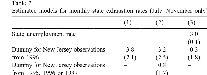
models are reported in Table 2. The first specification includes only a single dummy for New Jersey observations from 1996. This model provides a valid impact estimate under the assumption that exhaustion rates in New Jersey would move in parallel with the average changes in other states in the absence of NJEB. The estimated impact, 3.8%, is very similar to the averaged difference-in-differences estimate for New Jersey relative to the US as a whole in Table 1. Column (2) includes a second dummy variable for New Jersey data in 1995–1997. With this dummy included, the 1996 dummy measures the deviation of 1996 rates from the average of 1995 and 1997 rates, and is therefore conceptually similar to the averaged difference-in-difference estimate in Table 1. This change in spe-cification has little effect.
Columns (3)–(5) present models that include the state unemployment rate as a control variable for cyclical conditions in the labor market. This variable is strongly correlated with exhaustion rates, and its addition significantly reduces the standard error of the regression models, albeit at the cost of some potential endogeneity bias. Controlling for state unemployment, the estimated impact of
22
Table 2
a Estimated models for monthly state exhaustion rates (July–November only)
(1) (2) (3) (4) (5)
State unemployment rate – – 3.0 3.0 3.0
(0.1) (0.1) (0.1) Dummy for New Jersey observations 3.8 3.2 0.3 2.4 2.4
from 1996 (2.1) (2.5) (1.8) (2.2) (2.2)
Dummy for New Jersey observations – 0.8 – 22.5 22.5
from 1995, 1996 or 1997 (1.7) (1.5) (1.5)
Monthly trend for New Jersey 2 2 2 2 0.1
observations in 1996 only (1.2)
2
R 0.65 0.65 0.73 0.73 0.73
Standard error of regression 6.0 6.0 5.3 5.3 5.3
a
Standard errors in parentheses. Estimated on sample of 3136 monthly observations for 49 states for July–November of 1985–1997. (Data for November 1997, and for Idaho and New Hampshire, are unavailable.) The dependent variable is the seasonally adjusted monthly state exhaustion rate (in percentages). Models include unrestricted state and year effects. Monthly trend variable is normalized to have mean 0 over the July–November 1996 period.
NJEB (i.e. the 1996 New Jersey dummy) is somewhat sensitive to the inclusion of the 1995–1997 dummy, although the estimates are still quite imprecise. Finally, in column (5) we include a monthly trend variable that increases linearly over the July–November 1996 period. (For ease of interpretation this trend variable has a mean of 0.) This term allows us to test for any systematic trend in the relative New Jersey exhaustion rate during 1996. As suggested by the patterns in Fig. 3, the estimated trend is positive, although very imprecisely estimated.
Overall, the results in Tables 1 and 2 suggest that there was a modest increase in exhaustion rates in New Jersey during the period that UI claimants were eligible for extended benefits — of the order of 1–3 percentage points. However, given the rather large month-to-month variability in state-level exhaustion rates, we cannot rule out an effect of 0, or one as large as 6–8 percentage points.
5.2. Analysis of administrative records
We turn now to a more detailed analysis of individual UI claim data from New Jersey during the 1995–1997 period. As noted earlier, an implicit assumption throughout this analysis is that claimants who were scheduled to exhaust in the July–November period in 1996 were comparable to those claimants in a pooled 1995 / 1997 sample from the same months with the exception of NJEB eligibility. Weak evidence in favor of this hypothesis is provided by the similarity of the impact estimate in Table 1 that uses only New Jersey data [i.e. the estimate in the bottom row of column (1)] to estimates that use either Pennsylvania or other US states as a comparison group.
D
Characteristics of UI recipients in NJ, by potential exhaustion date
July 1–November 24 Difference: 199621995 / 1997 average
1995 1996 1997 Difference t-statistic
Unemployment rate (county) 6.9 7.0 5.8 0.7 78.00
Average weekly wage 572 567 572 25.0 3.37
Replacement rate 53.7 53.9 54.5 20.2 2.79
Age at claim date 38.9 39.0 39.2 0.0 1.61
White (not Hispanic) (%) 64.4 62.3 60.2 0.0 0.08
Black (not Hispanic) (%) 16.0 17.3 18.4 0.1 1.01
Hispanic (%) 16.8 17.5 18.3 20.1 0.41
Female (%) 35.2 37.0 37.8 0.5 2.86
Years of education 12.26 12.27 12.27 0.0 0.66
Union member (%) 15.9 15.6 14.9 0.2 1.13
US citizen (%) 86.4 86.1 86.0 20.1 0.83
Weeks worked for former employer 49.4 53.6 51.0 3.4 11.58
Industry distribution(%)
Agriculture 2.8 2.4 2.9 20.5 7.26
Mining 0.3 0.3 0.2 0.1 3.84
Construction 17.4 15.5 14.9 20.7 4.45
Manufacturing 19.6 18.8 17.9 0.1 0.02
Transportation and public utilities 6.0 6.6 6.6 0.3 3.80
Wholesale trade 8.1 8.5 8.6 0.2 0.73
Retail trade 13.3 15.3 14.5 1.4 10.30
Finance, insurance and real estate 5.7 4.8 4.9 20.5 5.29
Public administration 2.2 2.0 2.0 20.1 2.35
Services 23.9 25.1 27.2 20.5 2.91
UI claim characteristics
Percentage eligible for 26 weeks of regular UI 68.3 70.4 67.7 2.7 13.23
Average weeks of UI received 17.6 16.9 16.4 20.3 1.75
Percentage exhausted regular UI 48.5 47.1 42.9 0.8 7.29
Percentage received NJEB 2.3 31.6 0.0 30.3 204.70
Number of observations 89 226 103 492 90 590 2 2
a
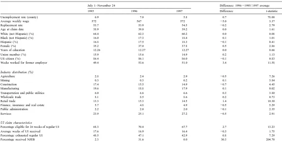
comparison for the 1996 claims sample is provided in Table 3, where we present a variety of descriptive statistics for 1995, 1996 and 1997 claims, along with t-tests for the hypothesis that the 1996 mean is the same as the average in 1995 and
23
1997. The first row presents county level unemployment rates (at the first
payment date for each claim). By this measure, economic conditions were fairly
24
stable between 1995 and 1996 before improving in 1997. Other than this change,
the characteristics of New Jersey UI claimants were fairly stable over our sample period. Nevertheless, the large samples provide very precise estimates, so many of these small differences are statistically significant, as indicated by the t-statistics in
25
the fifth column of the table.
The bottom panel of Table 3 displays UI claim characteristics over the three periods. Just over two-thirds of recipients are eligible for the full 26 weeks of regular benefits in each year. The percentage of recipients that exhausted their regular benefits in each period is very similar to the aggregate exhaustion rates reported in Table 1, indicating that the bias introduced in the aggregated data by using a potentially mis-measured denominator is small. A comparison of the 1996 rate to the average of 1995 and 1997 indicates that the percentage of respondents that exhausted their regular benefits climbed 0.8 points in response to NJEB. This difference may be attributable to the availability of extended benefits or, alternatively, to the relatively higher rate of unemployment in 1996 compared to the 1995 / 1997 average. Almost one-third of respondents in the 1996 sample
26
collected extended benefits.
23
Ninety-four percent of claims that were scheduled to exhaust in the period June–November, 1996, were filed before June 2, 1996 (the effective date of NJEB). Thus, there is little likelihood that the composition of the claims sample was directly affected by NJEB.
24
The average county unemployment rates are higher than the state averages in Fig. 1 because the administrative records sample over-weights counties with higher unemployment. Similar weighting issues may also explain the fact that the state average unemployment rate is slightly higher in 1995 than 1996, but no difference is observed here. Although one would expect the sample sizes in 1995 and 1996 to be larger than that for 1997 based on the unemployment rates across years, the number of observations available for 1995 is diminished somewhat by the sample design. Some individuals filing an initial claim towards the end of 1994 might not receive a first payment until sometime in 1995 if there was some question regarding his / her eligibility for benefits and could have potential exhaustion dates between July and November of that year. Because our sample consists of initial claims filed on or after January 1, 1995, these claimants are not in our data.
25
The standard errors reported here, and in the remainder of our analysis, are subject to some understatement because they do not incorporate the correlation that may exist across observations within a particular geographic region at a point in time. In our analysis of state-level data, we estimated comparable models to those reported in Table 2 but controlled for the correlation across monthly observations within states and years and found no substantive changes in statistical inference. For instance, using the ‘cluster’ option in Stata to estimate the model in Table 2, column (1) actually led to a reduction in the estimated standard from 2.06 to 2.05. We address the analogous issue using the micro-data later in the paper.
26
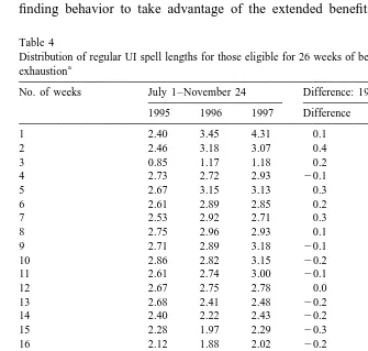
Table 4 presents the actual distribution of weeks of regular UI receipt for those recipients eligible for 26 weeks of benefits in each of the three sample periods. The proportion of recipients who exhausted their regular benefits is somewhat smaller here than reported in Table 3 because the full sample of spells (in Table 3) includes recipients eligible for fewer than 26 weeks of benefits, who are more likely to exhaust. Column (4) of Table 4, which compares the 1996 frequencies to the averages for 1995 and 1997, suggests that during the NJEB period there was a 1.5 percentage point increase in the share of spells that exhausted their regular benefits in 1996 compared to 1995 and 1997. Consistent with these findings, the share of recipients finding jobs in weeks 13–26 is slightly lower in 1996 compared to 1995 and 1997, indicating that some individuals may have shifted their job finding behavior to take advantage of the extended benefits. Again the relative
Table 4
Distribution of regular UI spell lengths for those eligible for 26 weeks of benefits, by potential date of a
exhaustion
No. of weeks July 1–November 24 Difference: 199621995 / 1997 average 1995 1996 1997 Difference t-statistic
26 (exhausted) 44.06 43.15 39.30 1.5 2.57
Number of observations 62 545 72 600 62 955 – – a
frequencies are precisely estimated, and many of the differences are statistically significant.
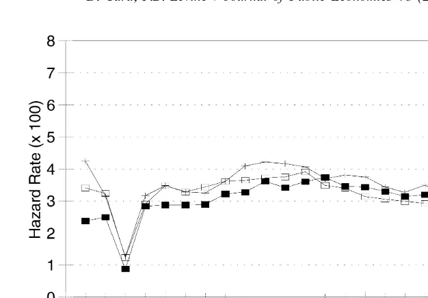
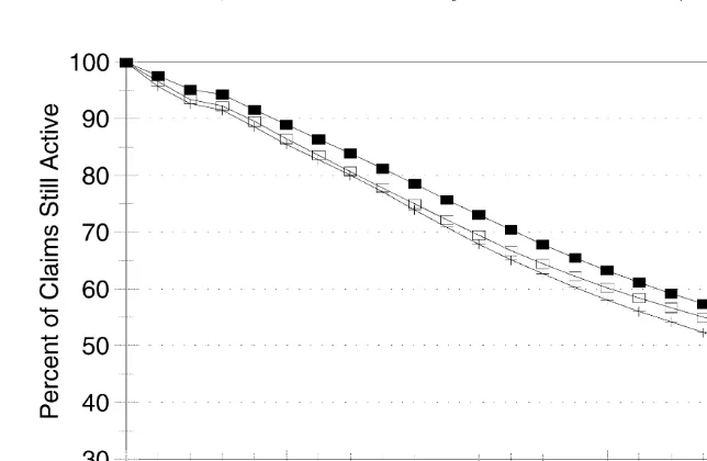
An alternative way to organize the same data is to construct the hazard rates out of UI (and the associated survivor functions) for UI recipients who were eligible
27
for 26 weeks of regular benefits before, during, and after NJEB. These are
graphed in Figs. 4 and 5. As in other administrative data bases, the New Jersey sample shows a notable ‘spike’ in UI-leaving rates just prior to regular benefit
28 29
exhaustion. Somewhat to our surprise, however, a fairly similar spike is also
apparent in 1996, when NJEB was in effect. The traditional interpretation of the rapid rise in UI exit rates just prior to exhaustion is that some UI recipients wait
30
until the ‘last minute’ to begin a new job (or begin searching for a new job). On
this basis, one might expect to see a much smaller spike at 25 weeks when NJEB were available. The presence of such a strong spike in our 1996 sample suggests that the rise in UI-leaving rates at week 25 in the 1995 and 1997 samples may be due in part to factors other than the strategic timing of job starting dates.
A close examination of the hazard rates in Fig. 4 reveals that although UI-exit rates in 1996 were between those in 1995 and 1997 for the first 12 weeks of claims, the 1996 hazard rates were lower than those in either 1995 or 1997 after the 13th week. Similarly, although the survivor function for 1996 claims is parallel to the function for 1997 for the first 10–12 weeks, after that point the two functions begin to diverge. After 13 weeks about 1.7% more claimants are still on
27
An alternative approach that would utilize all spells would be to create hazard rates by ‘weeks until exhaustion,’ which should show a spike within the few weeks prior to the regular benefit cut-off. We experimented with these hazards and found similar patterns to those reported here. We chose to report hazard rates by weeks unemployed among a sample of recipients eligible for a uniform 26 weeks because it is easier to interpret.
28
Because of data limitations, the actual spike is probably somewhat more muted than that presented here. All the statistics reported in this paper refer to full weeks of benefit receipt. Yet the administrative data from which our statistics are derived enumerate calendar weeks, in which any benefit received during the week is counted. Although we can largely correct for this distinction, we cannot identify those recipients whose first calendar week of benefits was a partial week. Therefore, for some recipients our count of full weeks of benefit receipt is overstated by one. If, for example, a claimant became unemployed in the middle of a week and started a new job on a Monday, the measured number of calendar weeks of benefits received will be one higher than the number of full weeks and we are unable to correct for this. Individuals who are coded in our data as leaving UI in the week just prior to benefit exhaustion may have actually collected only 24 weeks of full regular benefits. This problem leads to some overstatement of the pre-exhaustion exit spike. We are unsure whether a similar issue may be present in earlier data sets.
29
The downward spike at 3 weeks reflects the fact that recipients are paid the weekly benefit for the initial waiting week if their spell extends to 4 weeks or longer. Therefore, the marginal benefit of remaining unemployed from the third to the fourth week is really 2 weeks’ worth of benefits, not 1. Standard search models would predict such an incentive would lower the hazard rate in the third week and this prediction appears to be verified in the data.
30
Fig. 4. Hazard rates out of regular UI receipt.
UI in 1996 than in 1997. But by the 25th week, this gap has risen to 4 percentage points.
In interpreting this apparent ‘twist’ in the 1996 hazard rate relative to the 1995 or 1997 rates, it is important to keep in mind that most claim spells in our 1996 sample were in progress when the NJEB program was announced. Indeed, among the subset of the 1996 sample eligible for 26 weeks of regular benefits, the median claimant would have been in his / her 13th week of UI on June 2, 1996 (had he / she not left UI). If the announcement of NJEB caused UI claimants to reduce their search intensity, one would expect to see a gradual downward shift in the average 1996 hazard from earlier claim weeks (which mostly occurred before the NJEB program was announced) to later claim weeks (which were increasingly likely to have occurred after the program was announced). Evidence from the hazard models presented below suggests that this is indeed a reasonable description of the program’s effect.
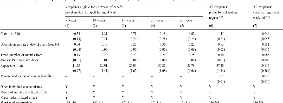
Before turning to the hazard models, however, we present a variety of simpler probit and censored normal regression (‘Tobit-style’) models for the determinants of the length of completed regular UI spells in our 1995–1997 samples. These models, which are presented in Table 5, can be interpreted as models for the latent
Fig. 5. Survivor function for regular UI spells.
individual will collect UI. The models in columns (1)–(5) of Table 5 are all
models for the event that y exceeds a given threshold (5, 10, 15, 20 or 26 weeks)i
conditional on eligibility for 26 weeks of regular benefits. The model in column
(6) describes the event that y exceeds the individual’s maximum weeks ofi
eligibility (M ), and is fit over the entire sample of claimants with potentiali
exhaustion dates between July and November of 1995, 1996 and 1997. Finally, the
model in column (7) is a censored normal regression model for y , taking intoi
account that yi#M . The latter model is interesting in part because similar modelsi
have been fit in the previous literature, allowing us to draw comparisons between the New Jersey claimant sample and earlier samples.
Card
,
P
.B
.
Levine
/
Journal
of
Public
Economics
78
(2000
)
107
–
138
129
a Determinants of regular UI spell length (probit derivatives multiplied by 100, standard errors in parentheses)
Recipients eligible for 26 weeks of benefits, All recipients: All recipients:
probit models for spell lasting at least: probit for exhausting censored regression
regular UI weeks of UI
5 weeks 10 weeks 15 weeks 20 weeks 26 weeks
(1) (2) (3) (4) (5) (6) (7)
Claim in 1996 20.54 21.21 20.71 0.18 1.62 1.45 0.044
(0.14) (0.21) (0.24) (0.25) (0.24) (0.21) (0.055)
Unemployment rate at date of claim (county) 0.04 0.18 0.28 0.36 0.23 0.53 0.151
(0.04) (0.05) (0.06) (0.06) (0.06) (0.05) (0.014)
Trend (number of months from 20.13 20.20 20.23 20.24 20.25 20.30 20.086
January 1995 to claim date) (0.01) (0.01) (0.01) (0.01) (0.01) (0.01) (0.003)
Replacement rate 11.23 20.91 25.07 30.21 32.79 37.20 10.114
(0.97) (1.41) (1.62) (1.68) (1.66) (1.34) (0.364)
Maximum duration of regular benefits – – – – – 22.52 20.033
(0.04) (0.010)
Other individual characteristics Y Y Y Y Y Y Y
Month of initial claim fixed effects Y Y Y Y Y Y Y
Major industry fixed effects Y Y Y Y Y Y Y
Number of observations 193 116 193 116 193 116 193 116 193 116 280 308 280 308
a
previous employer, and a set of major industry fixed effects. In the models in columns (6) and (7) we also include the individual’s maximum weeks of UI
31
entitlement.
The pattern of coefficient estimates for the NJEB-eligible dummy in Table 5 suggest that although UI claims with scheduled exhaustion dates after July 1, 1996
were somewhat less likely to survive 5, 10 or 15 weeks than comparable spells in]
1995 and 1997, they were somewhat more likely to survive 26 weeks, or to]]
32
exhaust. These findings mirror the pattern of the unadjusted survivor functions in
Fig. 5. In particular, up to about 15 weeks the survivor function for 1996 spells is somewhat below an average of the survivor functions for 1995 and 1997 (implying that 1996 spells were less likely to survive than spells in the pooled comparison group of 1995 and 1997 spells). Thereafter, however, the 1996 survivor function is above the average for 1995 and 1997 (implying that 1996 spells were more likely to last over 20 weeks or to exhaust than an average of 1995 and 1997 spells).
Reflecting the fact that 1996 spells were more likely to end quickly, but also more likely to exhaust, the estimates of the censored normal regression model in column (7) imply that on balance the number of weeks of regular benefits received by 1996 claimants was not too different from the average in 1995 and 1997. Several other aspects of the estimates from this model are also worth noting. For example, the estimated coefficient of the replacement rate variable implies that a 10 percentage point increase in the replacement rate (e.g. from 0.4 to 0.5) would increase the average duration of UI spells by about one week. This finding is comparable to estimates in the previous literature (see, for example, Mortensen, 1986; Meyer, 1990). The signs of the coefficient estimates for the censored normal model are consistent with those of the probit model for exhaustion, and the magnitudes of the coefficient estimates in the two models are also roughly consistent, suggesting that the normality assumption used in these models, although surely incorrect, does not affect the qualitative inferences from the
33
models.
31
In the probit model for exhaustion in column (6), note that the probability of exhaustion is
pi5P( yi.M ). If yi i5xib 1Mia 1u , and u is normally distributed with mean 0 and standardi i deviations, then pi5F(x (i b/s)2M (1i 2a) /s).
32
As indicated earlier, the standard errors reported here are subject to some understatement because they do not incorporate the correlation that may exist across observations at a point in time. This bias is probably larger in models that exclude the county-level unemployment rate, since the latter presumably accounts for some of the correlation across individuals. We re-estimated some models excluding the county unemployment rate and found that the standard errors on our key variables were only raised by 3–4% (the coefficient estimates are also not much affected), suggesting that local shocks are small relative to other variance components. In light of the relatively small standard errors for the estimates of the key parameters in our models, any bias caused by common local shocks would have to be quite large to affect our inferences; nevertheless, readers should be aware of this potential problem.
33
As we noted in the discussion of the hazard rates and survival functions in Figs. 4 and 5, most of the UI claims in our 1996 sample were actually in-progress when the NJEB program was announced. For this reason, it is likely that the estimates in Table 5 understate the ‘long-run’ effect of a 13-week benefit extension on the distribution of UI claims. Moreover, there is some evidence that UI claims in our 1996 sample were more likely to end early than those in a pooled sample of 1995
and 1997 claims. Since the early weeks of the 1996 claims were largely before the]]
NJEB program, it seems implausible that UI-leaving behavior in these weeks was affected by NJEB. Rather, we conjecture that economic conditions in early 1996 may have been somewhat ‘better’ than the average conditions in 1995 and 1997, leading to a somewhat higher exit rate from UI and an increase in the fractions of claims ending in 5 or 10 weeks in 1996, relative to the 1995 / 1997 comparison sample. If true, this suggests that the estimates in Table 5 (and those in our aggregate analysis in Tables 1 and 2) may understate even the ‘short-run’ impact of the NJEB program.
In light of the fact that almost all UI claim spells affected by the NJEB program were in-progress in June 1996, we turn to a hazard modeling framework for refining our estimates of the impact of the program. Specifically, we fit
discrete-time hazard models for the probability l(i,t) that individual i exits UI in week t,
conditional on having remained on UI up to week t21. We experimented with
both conventional proportional hazard models and a simple logit functional form,
34
and found very similar estimates from the two alternatives. For simplicity, we
report only the estimates from the logit specifications here. Since the probability of exiting UI in any given week is small (3.24%), the logit coefficient estimates show the approximate percentage change in the exit probability per unit change in the associated covariate.
A key advantage of the hazard framework is that it allows us to measure the effect of covariates whose values change over time, including the unemployment rate and most importantly the presence of the NJEB program. We therefore include in our hazard models two dummy variables: one indicating spells from our 1996 sample, and a second indicating whether the current week is after July 1, 1996. The former measures any differences in UI leaving rates between 1996 UI spells and those in the comparison sample of 1995 and 1997 spells, during all weeks of
these spells. The latter measures any differential change in UI leaving rates for the
1996 spells after the NJEB program was in place (allowing a month for information about the program to disseminate). In this specification, any un-observed factors that happened to shift UI leaving rates in 1996 relative to the average rate in 1995 and 1997 will be absorbed by the 1996 spell dummy, while
34
The standard proportional hazard specification is l(i,t)512exp(2exp( g(x )i 1h(t))). The logit
specification is log(l(i,t) /(12l(i,t)))5g(x )i 1h(t). As shown in Allison (1982), these specifications
D Hazard models of exit from unemployment insurance receipt (logit coefficients multiplied by 100, standard errors in parentheses)
20% sample 20% sample 20% sample Construction Union
only only
(1) (2) (3) (4) (5)
Claim in 1996 20.80 4.73 4.84 18.10 7.30
(1.26) (1.49) (1.49) (1.57) (1.68)
Claim in 1996* current week after – 216.62 216.25 222.39 217.37
July 1, 1996 (2.45) (2.72) (3.53) (3.32)
Claim in 1996* 1 week to exhaustion – – 2.38 27.84 216.79
(5.44) (7.09) (7.07)
Claim in 1996* 2 weeks to exhaustion – – 20.63 214.59 213.55
(7.27) (9.07) (9.04)
Claim in 1996* 3 weeks to exhaustion – – 211.66 1.79 8.18
(7.44) (8.82) (8.78)
Unemployment rate (county) 25.15 25.17 25.17 23.31 21.79
(0.36) (0.36) (0.36) (0.40) (0.41)
Replacement rate 2100.56 2100.79 2100.78 27.31 2123.30
(8.39) (8.39) (8.39) (11.75) (11.73)
Other individual characteristics Y Y Y Y Y
Number of observations (weeks at-risk) 907 476 907 476 907 476 498 077 552 906
a
the ‘pure’ effect of the NJEB program on UI leaving behavior will be measured by the time-varying post-NJEB coefficient.
Our hazard model estimates are presented in Table 6. For ease of computation we selected a random 20% subset from the overall sample of UI claims with scheduled exhaustion dates from July 1–November 24 of 1995, 1996 and 1997. This sample of 56 262 claims yields a total of 932 959 claim-weeks, including 25 283 ‘final payment’ weeks (weeks in which claimants exhaust their UI
35
entitlement), which are treated as right-censored observations. The risk set for
our hazard analysis therefore contains 907 476 observations. In light of the time pattern of the hazards shown in Fig. 4, we include a variety of controls for the ‘baseline’ exit probabilities: dummies for the first 3 weeks of regular UI receipt; a cubic in the number of elapsed weeks of regular UI receipt; and dummies for each
36
of the last 3 weeks prior to regular benefit exhaustion. We also experimented
with a variety of other controls, including linear and quadratic terms for the number of weeks remaining until exhaustion. The addition of such terms had essentially no effect on the estimates of the NJEB program impacts nor of the effects of the other covariates.
The specification in column (1) includes a single dummy variable for 1996 claims, along with the same set of individual covariates used in the models in Table 5. The estimate of the 1996 effect is negative, but small, and statistically insignificant. The effects of the control variables are typically significant, and consistent with the signs of the coefficients of the models in Table 5.
The specification in column (2) adds the second dummy variable which equals 1 for 1996 claim weeks after July 1. In this model the ‘1996’ effect is positive — indicating a 4.7% higher exit rate among 1996 spells than in the comparison sample of 1995 and 1997 spells — while the ‘post-NJEB’ effect is negative — indicating a 16.6% drop in the UI leaving rate once the NJEB program was in place. The pattern of these estimates provides a simple interpretation of the average hazards graphed in Fig. 4 and the probit results in Table 5. Specifically, the positive coefficient for 1996 spells suggests that prior to passage of NJEB, UI-leaving rates in 1996 were slightly higher than those in the 1995 / 1997 sample. On average, the earlier weeks in the 1996 claims sample occurred prior to NJEB, and the overall hazard rate was above the average 1995 / 1997 rate (as shown in Fig. 4), leading to somewhat fewer spells lasting longer than 5, 10 or 15 weeks (as shown by the probit models in Table 5). The availability of NJEB, however, led to a drop in UI leaving rates, causing a gradual drop in the average hazard among
35
For individuals who contributed two or more claims to our sample, we included only the first claim. This eliminated about 2% of all claims.
36
later weeks in the 1996 (which were more and more likely to have occurred after June), and leading to an increase in the fraction of spells that exhausted (as shown by the probit models for exhaustion).
The model in column (3) adds three additional variables, representing interac-tions of the post-NJEB dummy with the dummies for periods 1, 2 and 3 weeks just prior to regular benefit exhaustion. The estimated coefficients on these interaction terms are small and individually and jointly insignificant, suggesting that availabil-ity of NJEB led to only small changes in the size of the ‘spike’ in exit rates prior
37
to exhaustion.
The models in Table 6 all ignore the presence of unobserved individual-specific
38
heterogeneity. To get some sense of the possible implications of this omission,
we performed a number of checks. First, we estimated the models without any individual-specific covariates, to gauge the sensitivity of our estimates to
observ-able heterogeneity. This yielded estimates of the remaining baseline and NJEB
coefficients very similar to the ones from the richer specifications reported in the table. For example, with no individual-specific controls, the estimate of the 1996 dummy in a specification similar to the one in column (2) is 7.4 (vs. 4.7 with all
controls), while the estimate of the post-NJEB dummy is 218.7 (vs. 216.6 with
all controls). These results suggest that our estimates are not very sensitive to controlling for observed heterogeneity and, therefore, may not be terribly sensitive to unobservable heterogeneity either. Second, we compared the observable characteristics of individuals ‘at risk’ to leave UI after various numbers of weeks. These comparisons show surprisingly little systematic trend with time on UI. For example, average education is 12.3 years in week 1, 12.3 years in week 12, and 12.4 years one week prior to exhaustion of regular benefits. Similarly, the mean log average weekly wage (for the old job) is 6.16 in week 1, 6.14 in week 12, and 6.13 one week prior to exhaustion. Based on these results for the observable covariates, we think it is unlikely that unobserved characteristics lead to much bias in our estimates of the impact of NJEB.
Another concern with the results in Table 6 is that our estimates of the impact of NJEB are heavily based on the effect of NJEB on later weeks of long spells (since the average benefit week ‘at risk’ in the post-NJEB period of 1996 is about week 15). This is only a problem, of course, to the extent that the post-NJEB effect varies with spell duration, or varies across spells by the duration of the completed spell. To assess the possible magnitude of this type of heterogeneity, we
37
In this specification, the indicator variables for the weeks immediately preceding exhaustion do not also need to be interacted with a post-implementation dummy variable because all those eligible for NJEB with potential exhaustion dates beyond July 1 would have approached their last few weeks of eligibility after June 2.
38
augmented the basic specification in column (2) with an interaction between the post-NJEB dummy and a quadratic in the elapsed spell duration. The resulting interactions are at best marginally significant, and show only a small increase in the NJEB effect with elapsed duration. We also tried an ad hoc re-weighting scheme to evaluate the average effect of NJEB if the distribution of weeks at risk for the NJEB ‘treatment’ was representative of the overall distribution of weeks at risk to exit UI. Specifically, for each person-week ‘at risk’ to leave UI in the post-NJEB 1996 sample, we weighted the observation by the ratio of the relative number of person-weeks of the same elapsed duration in the 1995 / 1997 com-parison sample to the relative number in the post-NJEB 1996 sample. We then fit the duration model by weighted logit. The resulting estimate of the post-NJEB
coefficient was 217.9 (vs. the unweighted estimate of 216.6). Based on these
results we conclude that any effects of heterogeneity in the NJEB effect are small. As indicated earlier, another issue regarding the NJEB program is that some UI recipients may have been unaware of their eligibility for the program. To address this, we replicated our analysis on two subgroups of workers that we suspect were relatively well-informed about the program: union members (whose leaders lobbied for the extension); and workers in the construction industry (who are much more likely to be ‘repeat’ users of UI — cf. Meyer and Rosenbaum, 1996). Estimation results for these groups are shown in columns (4) and (5) of Table 6. Interestingly, the estimated effects of NJEB for these subgroups are quite similar to those obtained for the overall sample. In particular, the announcement of NJEB seems to have lowered exit rates by about 20% for both groups, with little indication of any effect on the size of the ‘pre-exhaustion’ spike.
6. Discussion and conclusions
Taken as a whole the results of our analysis provide two alternative views of the effect of the 1996 benefit extension in New Jersey. Overall, the NJEB program appears to have had a very modest impact on UI claim behavior in the state. The fraction of recipients who exhausted regular benefits increased by about 1.5 percentage points and the average spell length was largely unchanged [Table 5, columns (5)–(7)]; while the average exit rate from regular UI was only marginally affected [Table 6, column (1)]. Our reading of the evidence is that this modest program impact was due to the short-term nature of the program. Many NJEB-eligible recipients spent a large share of their unemployment spell looking for work before NJEB was introduced. Moreover, in the absence of NJEB it appears that UI spells in New Jersey in 1996 would have been slightly shorter than spells in our comparison sample of 1995 and 1997 spells. In hazard models that measure the impact of NJEB on weeks of claim recipiency after the program was
suggest that the entire hazard profile shifted down by about 17% in each week following the onset of the extended benefit program [Table 6, column (2)].
We used this estimate to simulate the ‘long-run’ effect of a 13-week benefit extension on a pool of unemployed workers who were eligible for 26 weeks of regular benefits and knew from the start of their spell that they could receive extended benefits. Starting with the sample of 1997 UI claimants as a reference population, we calculated claim survivor functions assuming that the weekly hazard rates were 16.6% lower than the observed rates. The results of the simulation suggest that the ‘long run’ effect of a 13-week extended benefit program would be a 7 percentage point increase in the regular UI exhaustion rate, and a roughly 1 week increase in the average number of weeks of regular UI collected by claimants. The latter estimate of the sensitivity of weeks of regular UI receipt to average benefit duration is lower than the estimate reported by Katz and Meyer (1990a), whose results suggest that a 13-week benefit extension should
39
increase spell lengths by 2–2.5 weeks.
Although the evidence from the 1996 NJEB program suggests that exit rates from regular UI are significantly affected by a benefit extension, there is no indication that the availability of extended benefits has much affect on the rise in UI-leaving rates in the weeks just prior to the exhaustion of regular benefits. This finding raises an important question regarding the cause of the pre-exhaustion spike in exit rates. It is still possible that this spike is caused by the existence of a UI system that typically offers regular benefits for 26 weeks. For instance, Topel (1983) argues that employers enter into implicit contracts with workers and cycle them through spells of unemployment to extract the surplus created by imperfect experience-rating in the financing of UI benefits. If the terms of the agreement include a 26-week spell of unemployment, then changing these contractual arrangements in response to a short-term policy may be impractical. Alternatively, workers may have been conditioned to become less selective regarding possible job opportunities around the time that UI typically expires. Again, a longer-term policy might be expected to have a bigger effect on the size of the pre-exhaustion spike than a short-term policy like NJEB. Other explanations may be available, but regardless, the evidence indicates that at least a short-term benefit extension has little or no impact on that spike.
These considerations also suggest that even our long-term estimates of the effect of a 13-week extended benefit program may be understated. If the program was in
39